If you need a quick way to check whether a cell is truly empty, the ISBLANK function is what you reach for.
It returns TRUE when a cell holds nothing at all and FALSE the moment there’s a value, a space, or even a formula that returns an empty string.
In Excel 365, you can also feed ISBLANK a range and the results spill into the cells below. In this article, I’ll walk you through how ISBLANK works with a few practical examples.
ISBLANK Function Syntax in Excel
Here is the syntax of the ISBLANK function:
=ISBLANK(value)
- value – The value you want to test. This is usually a cell reference, but it can also be a range in Excel 365. ISBLANK returns TRUE only when the referenced cell is genuinely empty, and FALSE for anything else.
One thing worth knowing right away. ISBLANK is strict about what counts as “blank”. A cell with a space character in it, a cell with a formula that returns "", or a cell with any value at all returns FALSE. Only a cell that was never touched (or was cleared with Delete) returns TRUE.
When to Use ISBLANK Function
Use this function when you need to:
- Flag rows that are missing a required value
- Drive an IF formula off whether a cell has been filled in
- Count how many cells in a range are still empty
- Pull a clean list that skips the blank rows
- Tell the difference between a truly empty cell and one that just looks empty
Let me show you a few practical examples of how to use ISBLANK.
Example 1: Flag Empty Cells in a Column
Let’s start with the most basic use of ISBLANK.
Below is the dataset. I have a list of customer names in column A, but a few rows were left empty. I want a TRUE or FALSE next to each row so I can see at a glance which cells are missing a name.
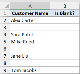
I want column B to show TRUE for every empty cell in column A and FALSE for every cell that has a name in it.
Here is the formula:
=ISBLANK(A2:A9)
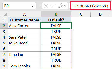
In the above formula, I’m feeding ISBLANK the entire range A2:A9 in one shot. Since ISBLANK spills in Excel 365, you only need to type the formula once in cell B2 and the results fill down to B9 automatically.
The rows where the name is missing return TRUE. The rows that have a name return FALSE. Notice that ISBLANK doesn’t care what the value is. A name, a number, a date, or even a single space would all return FALSE.
Pro Tip: If you are on an older version of Excel that does not support dynamic arrays, type =ISBLANK(A2) in B2 and drag it down through B9. Same result, just the legacy way of doing it.
Example 2: Mark Order Status Based on Blank Dates
Here’s where ISBLANK starts to feel useful in a real workflow.
Wrapping ISBLANK inside an IF formula lets you read off the state of one column and stamp a label in another. It’s the standard way to drive a “Pending vs Delivered” style status off whether a date has been filled in yet.
Below is the dataset. I have a list of orders in column A and their delivery dates in column B. Orders that haven’t shipped yet have an empty date cell. I want column C to show “Pending” for those and “Delivered” for the rest.
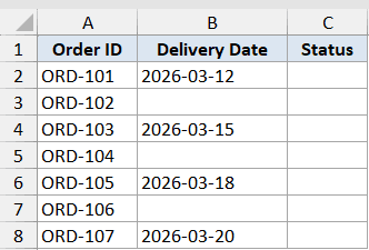
I want column C to read the delivery date in column B and stamp the right status next to each order.
Here is the formula:
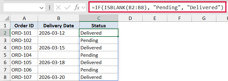
=IF(ISBLANK(B2:B8), "Pending", "Delivered")
How this formula works:
- ISBLANK(B2:B8) tests each delivery date cell. It returns TRUE for the rows where the date is empty and FALSE for the rows where a date is filled in.
- IF then picks the right label. TRUE means use “Pending”, FALSE means use “Delivered”.
- The result spills down column C, one status per order.
Orders with a date in column B get marked “Delivered”. Orders with an empty date cell get marked “Pending”.
Pro Tip: This approach only works when the empty cells are truly blank. If column B is pulling dates from another formula that returns "" for missing values, ISBLANK will return FALSE on those cells and your status column will get the wrong label. Example 4 covers that gotcha in more detail.
Example 3: Count Blank Cells in a Range
Sometimes you don’t need to label every row. You just need a single number that tells you how many cells are still empty.
Below is the dataset. I have a column of survey responses in column A. A few respondents skipped the question, so some cells are empty.
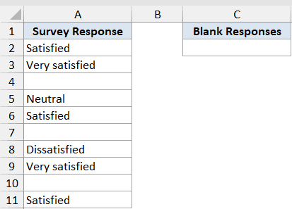
I want a single number in cell C2 that tells me how many survey responses are missing.
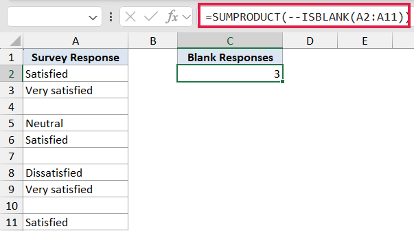
Here is the formula:
=SUMPRODUCT(--ISBLANK(A2:A11))
How this formula works:
- ISBLANK(A2:A11) returns an array of TRUE and FALSE values, one per row.
- The double minus (–) coerces those into 1s and 0s. TRUE becomes 1, FALSE becomes 0.
- SUMPRODUCT adds them up, giving you the count of blank cells.
In this example, the result is 3 since three respondents skipped the question and seven filled it in.
> COUNTBLANK is the more direct way to do this: =COUNTBLANK(A2:A11). The difference is that COUNTBLANK also counts cells that contain "" (an empty string returned by a formula), while SUMPRODUCT with ISBLANK only counts the truly empty cells. Pick the one that matches what you actually want to measure.
Example 4: ISBLANK vs the “” Gotcha
This is the example most people learn the hard way.
A cell can look empty without being empty. If another formula returned "" to a cell, the cell shows nothing on screen, but ISBLANK still returns FALSE because the formula counts as content. The ="" comparison, on the other hand, returns TRUE for both truly empty cells and cells holding "".
Below is the dataset. Column A has a mix of cells. Two are truly empty, two contain a formula that returns "", and two contain regular text.
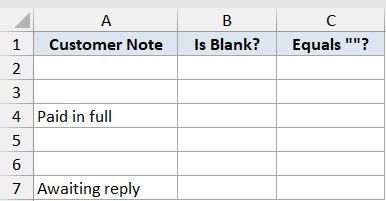
I want to compare ISBLANK and the ="" test side by side so the difference is obvious.
Here are the two formulas:
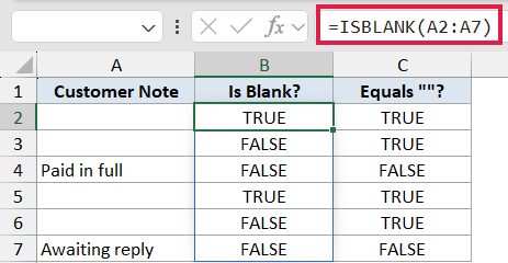
=ISBLANK(A2:A7)
=A2:A7=""
How this formula works:
- ISBLANK only returns TRUE when the cell is genuinely empty. The two rows that look empty but actually contain
=""return FALSE. - The
=""comparison returns TRUE for both truly empty cells and cells holding an empty string from a formula. - That gap is why a “Pending” status driven by ISBLANK can give the wrong label when your dates come from a lookup formula that returns
""for missing values.
If your column has formulas in it, the safer test is usually =A2="" or =LEN(A2)=0. If you specifically want to know whether the cell was ever filled in at all, ISBLANK is the one you want.
Pro Tip: If you’re not sure what’s in a cell, click it and check the formula bar. A truly empty cell shows nothing. A cell with "" shows the formula that produced it. A cell with a space shows a space (use Ctrl+End or zoom in if you can’t tell).
Example 5: Filter Out Blanks to Get a Clean List
Let’s wrap up with a useful spill formula.
Sometimes you don’t want flags or counts. You just want a clean list with the blanks stripped out. FILTER paired with NOT and ISBLANK does that in a single formula.
Below is the dataset. I have a list of sales leads in column A, but a few rows were left empty when the spreadsheet was put together. I want a clean list in column C that contains only the rows with a name in them.
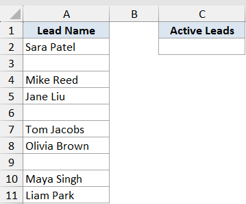
I want column C to pull just the active leads from column A and skip the empty rows.
Here is the formula:
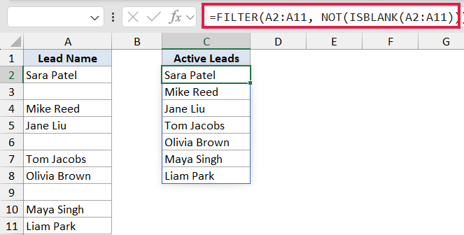
=FILTER(A2:A11, NOT(ISBLANK(A2:A11)))
How this formula works:
- ISBLANK(A2:A11) returns a TRUE/FALSE array. TRUE for the empty rows, FALSE for the rows with a name.
- NOT flips that array. TRUE becomes FALSE, FALSE becomes TRUE. Now TRUE marks the rows we actually want to keep.
- FILTER takes that TRUE/FALSE array as its include test and keeps only the rows where the test returns TRUE.
- The result spills into column C as a clean list of active leads with no gaps.
You get Sara Patel, Mike Reed, Jane Liu, Tom Jacobs, Olivia Brown, Maya Singh, and Liam Park stacked together in column C, with the three empty rows from column A dropped out.
Tips & Common Mistakes
- ISBLANK is strict about what counts as blank. Only a cell that’s truly empty returns TRUE. A space, a zero, an empty string from a formula, or any other value returns FALSE.
- A cell containing
=""is not blank to ISBLANK. This catches a lot of people. If your column is fed by a lookup or IF formula that returns""for missing values, ISBLANK returns FALSE on those cells. Use=A2=""or=LEN(A2)=0if you want both truly empty cells and""cells to count as blank. - COUNTBLANK and ISBLANK count different things. COUNTBLANK treats
""as blank. SUMPRODUCT with ISBLANK does not. Pick the one that matches your intent. - ISBLANK on a range returns an array. Feed it a single cell and you get a single TRUE/FALSE. Feed it a range in Excel 365 and it spills the results down the column. In older Excel versions, drag the formula down instead.
- Pair it with NOT to keep the non-blanks.
NOT(ISBLANK(...))is the cleanest way to say “this cell has something in it”. It’s the include test you reach for when filtering out empty rows. - Pair it with IF for status labels.
=IF(ISBLANK(B2), "Pending", "Delivered")is a very common workflow pattern. Just make sure the empty cells are actually empty and not the result of another formula returning"". - Watch out for spaces. A cell that visually looks empty but has a space character in it returns FALSE from ISBLANK. If you’re cleaning up imported data, run a TRIM pass first or use
=LEN(TRIM(A2))=0to catch both empties and whitespace-only cells.
That covers the main ways ISBLANK shows up in real spreadsheets. On its own it’s a one-line check for an empty cell. But pair it with IF to drive status labels, with SUMPRODUCT or COUNTBLANK to count missing values, or with FILTER and NOT to pull a clean list, and it quietly does a lot of work.
Related Excel Functions / Articles:
- COUNTA Function in Excel
- COUNT Function in Excel
- Count Cells that are Not Blank in Excel (Formulas)
- How to Highlight Blank Cells in Excel?
- How to Count Cells with Text in Excel?
- Remove Blank Rows in Excel (5 Ways + VBA)
- How to Remove Blank Columns in Excel? (Formula + VBA)
- Fill Blank Cells with 0 in Excel
- ISTEXT Function in Excel
- ISNA Function in Excel
- ISNUMBER Function in Excel