
Excel’s FALSE function returns the logical value FALSE. It takes no arguments, and typing FALSE directly produces the same logical value.
Although both can look identical in a worksheet, the logical value FALSE is different from the text value FALSE.
In this article, I’ll show you how to spot that difference, force an exact lookup, and use FALSE in status checks and calculations.
FALSE Function Syntax in Excel
The FALSE function has the following syntax:
=FALSE()
- FALSE takes no arguments. The empty parentheses are required when you use the function form.
- You can type FALSE without parentheses when you only need the logical value.
When to Use FALSE Function
- Enter a logical FALSE value in a cell or another formula.
- Require an exact match with VLOOKUP instead of its default approximate match.
- Count open, unchecked, or incomplete items stored as FALSE.
- Exclude nonmatching values from an array calculation without inserting zeros.
- Turn an amount off in arithmetic by multiplying it by a FALSE flag.
Example 1: Identify Logical and Text FALSE Values
Let’s start with a distinction that can prevent confusing formula results.
Below is the dataset showing four ways FALSE can appear. B2 holds typed FALSE, B3 uses =FALSE(), B4 uses =10<5, and B5 holds imported text.
Column C carries the header “Is Logical?” and will show the result for each entry.
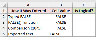
We want to check which entries are genuine logical values rather than text.
Here is the formula:
=ISLOGICAL(B2:B5)
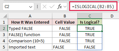
ISLOGICAL checks each cell in B2:B5 and spills TRUE, TRUE, TRUE, and FALSE into C2:C5.
The typed value, FALSE() result, and comparison result are logical values. The imported text only looks the same, so ISLOGICAL returns FALSE for B5.
Pro Tip: The text entry in B5 sits left-aligned, unlike the logical values. Treat that as a visual clue, then confirm it with ISLOGICAL.
Example 2: VLOOKUP Exact Match With FALSE
One common place to use FALSE is in VLOOKUP’s last argument.
Below is the dataset showing an auto-parts list with part numbers, descriptions, and list prices. A lookup card contains BR-1108 and an empty List Price result cell.
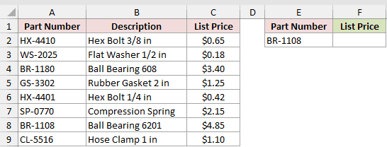
We want to return the list price for the exact part number entered in E2.
Here is the formula:
=VLOOKUP(E2,A2:C9,3,FALSE)
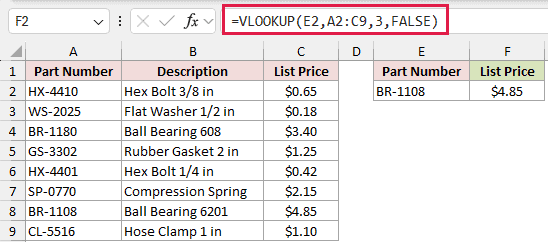
How this formula works:
- VLOOKUP searches the first column of A2:C9 for the part number in E2.
- The column index 3 tells Excel to return the matching value from the List Price column.
- FALSE requires an exact match, so VLOOKUP returns $4.85 for BR-1108 in row 8.
In Excel 2021 and later, XLOOKUP can handle this with =XLOOKUP(E2,A2:A9,C2:C9) and uses exact matching by default. VLOOKUP still works in older versions.
Pro Tip: Leaving VLOOKUP’s last argument out means approximate matching. Keep FALSE when you need the exact part number.
Example 3: Count FALSE Values With COUNTIF
Now let’s use FALSE as a criterion in a checklist.
Below is the dataset showing onboarding tasks, their owners, and logical values in the Done column. The Open Tasks result cell is blank.
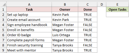
We want to count the tasks whose Done value is FALSE.
Here is the formula:
=COUNTIF(C2:C9,FALSE())
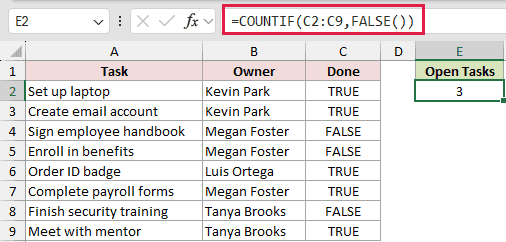
COUNTIF checks C2:C9 for logical FALSE values and returns 3. The open tasks are signing the handbook, enrolling in benefits, and finishing security training.
In Excel for Microsoft 365 and Excel for Microsoft 365 for Mac, the same pattern can count unchecked in-cell check boxes because their cells hold logical FALSE values.
Example 4: Use FALSE as Zero in Arithmetic
FALSE can also act as a simple on-or-off switch in a calculation.
Below is the dataset showing expenses, amounts, and Reimbursable flags. The Reimbursed Amount column will hold the calculated values.
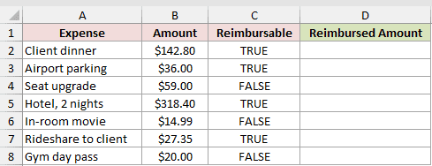
We want to keep each reimbursable amount and return zero for every nonreimbursable expense.
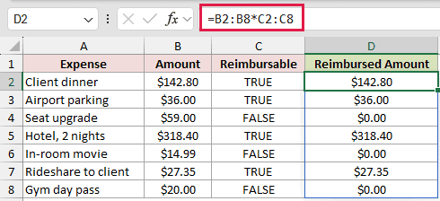
Here is the formula:
=B2:B8*C2:C8
How this formula works:
- B2:B8 contains the expense amounts.
- C2:C8 contains TRUE and FALSE reimbursement flags.
- In arithmetic, TRUE counts as 1 and FALSE counts as 0. Multiplication keeps reimbursable amounts and changes the others to $0.00.
The formula spills $142.80, $36.00, $0.00, $318.40, $0.00, $27.35, and $0.00 into D2:D8.
Spilling range formulas work in Excel 2021, Excel 2024, and Microsoft 365. In Excel 2019 and earlier, enter =B2:B8*C2:C8 across D2:D8 with Ctrl+Shift+Enter, or use one formula per row.
Example 5: Conditional Median With FALSE Instead of Zero
This final example shows why FALSE does not always behave like a stored zero.
Below is the dataset showing apartments, bedrooms, and monthly rents. The criteria card specifies 2 bedrooms, with empty Median Rent and Median Using 0 result cells.
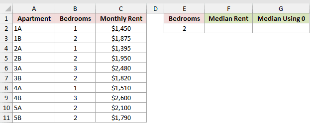
We want the median rent for 2-bedroom apartments, then compare FALSE with zero as the placeholder for nonmatching rows.
Here is the formula:
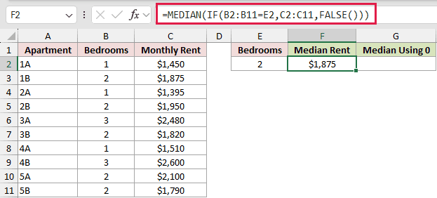
=MEDIAN(IF(B2:B11=E2,C2:C11,FALSE()))
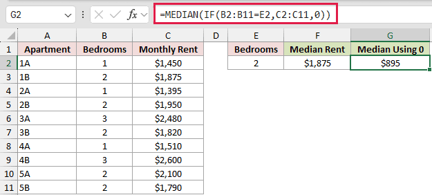
For comparison, here is the formula that substitutes zero:
=MEDIAN(IF(B2:B11=E2,C2:C11,0))
How these formulas work:
- B2:B11=E2 identifies the rows for 2-bedroom apartments.
- The first IF returns each matching rent and FALSE for every nonmatching row.
- MEDIAN ignores logical FALSE values inside the array, so the first formula returns $1,875.
- Replacing FALSE with 0 adds five zeros. The middle values become 0 and 1,790, so the second formula returns an incorrect $895.
In Excel 2021 and later, =MEDIAN(FILTER(C2:C11,B2:B11=E2)) is a more direct option.
MEDIAN(IF()) still works, including in Excel 2019 and earlier when entered with Ctrl+Shift+Enter.
Tips & Common Mistakes
- Do not confuse logical FALSE with imported or quoted text. ISLOGICAL confirms the type, while TYPE returns 4 for a logical value and 2 for text.
- FALSE() itself does not spill. ISLOGICAL in Example 1 and multiplication in Example 4 create the spilling results. A blocked spill range can produce a #SPILL! error.
- Avoid wrapping a comparison in IF just to return TRUE or FALSE. The comparison already returns the same logical result, which the NOT function can reverse when needed.
- If you omit IF’s value_if_false argument, Excel returns FALSE. Use
""when you want the formula to return blank text instead. - Do not assume FALSE always behaves as 0. Arithmetic coerces it to zero, but MEDIAN ignores logical values inside an array or reference.
I covered how the logical value FALSE differs from the text “FALSE” and how Excel handles it across these examples.
I hope you found this article helpful.
Related Excel Functions / Articles:
