
The SIN function in Excel returns the sine of an angle in radians.
For a right triangle, sine is the opposite side divided by the hypotenuse. That relationship helps calculate a height or another component of a measured length.
An angle measured in degrees needs conversion with RADIANS first.
In this article, I’ll show you how to calculate sine from degree measurements, find a ramp’s vertical rise, and convert results back to angles.
SIN Function Syntax in Excel
The SIN function takes one angle and returns its sine.
=SIN(number)
- number (required) is the angle in radians for which you want the sine.
When to Use SIN Function
- Find the sine of an angle that is already measured in radians.
- Convert angles in degrees and calculate their sine values.
- Calculate a vertical or opposite-side measurement when you know an angle and a hypotenuse.
- Create wave, rotation, or other periodic calculations.
- Check or reverse a sine calculation with related trigonometric functions.
Example 1: Find Sine From Degrees
Let’s start with the conversion you’ll use most often.
Below is the dataset. Column A lists eight angles measured in degrees, including angles beyond 180 degrees.
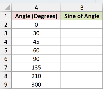
We want to convert every angle to radians and return its sine with one spilling formula.
Here is the formula:
=SIN(RADIANS(A2:A9))
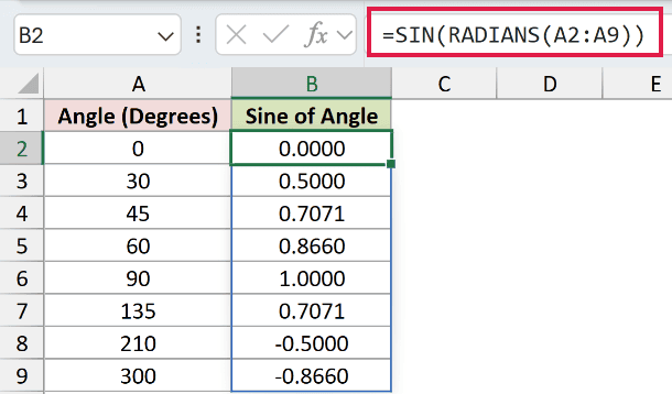
RADIANS converts the degree values first. SIN then calculates each result, and the eight values spill from B2 through B9.
The 30 degree row displays 0.5000, 90 degrees displays 1.0000, and 210 degrees displays -0.5000. SIN results always stay between -1 and 1.
Pro Tip: Keep the cells below B2 empty. If anything blocks B3:B9, Excel returns #SPILL! instead of placing the complete set of results.
Example 2: Why SIN(30) Is Not 0.5
Now let’s see what happens when you skip the conversion.
Below is the dataset. Column A contains eight angles from 10 to 75 degrees.
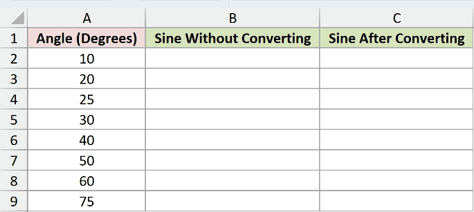
We want to compare SIN applied directly to those numbers with SIN after a degree-to-radian conversion.
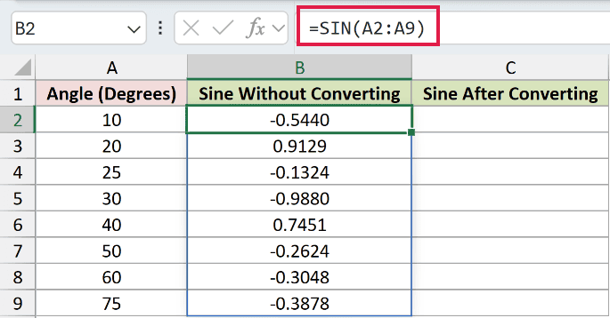
Here is the formula that skips the conversion:
=SIN(A2:A9)
And here is the longhand conversion using PI:
=SIN(A2:A9*PI()/180)
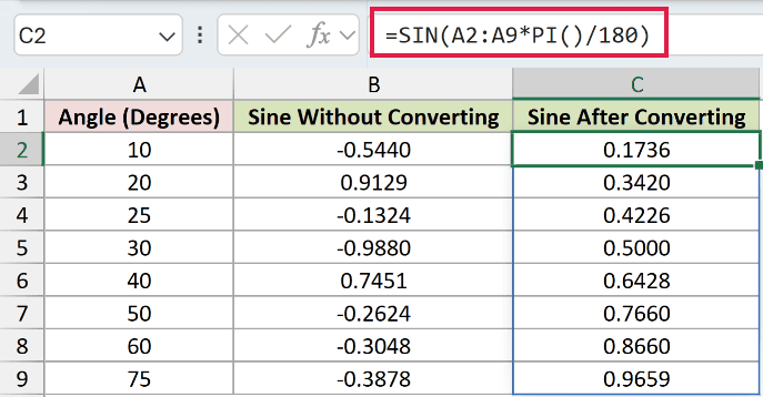
The first formula treats every number as radians. That is why 30 returns -0.9880 instead of the familiar 0.5000 shown after conversion.
Multiplying by PI and dividing by 180 performs the same conversion as RADIANS. The RADIANS version from Example 1 is shorter, but you’ll often see this longhand form.
Example 3: Calculate a Ramp’s Vertical Rise
Here’s one way to use the sine values.
Below is the dataset. It lists eight ramp IDs, their lengths in feet, and their incline angles in degrees.
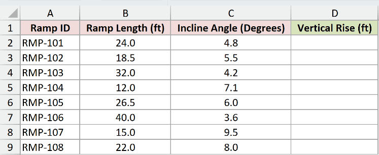
We want to calculate how much height each ramp gains from its length and incline angle.
Here is the formula:
=B2:B9*SIN(RADIANS(C2:C9))
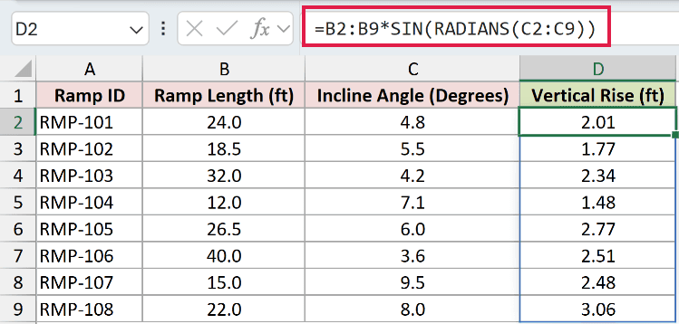
SIN returns the ratio between the vertical rise and ramp length. Multiplying that ratio by each length gives the rise in feet.
For RMP-101, a 24.0-foot ramp at 4.8 degrees gains 2.01 feet of height. The other results spill down through D9.
COS would calculate the horizontal run from the ramp length, while TAN works when you know the horizontal run. Neither replaces SIN for this setup.
Example 4: Handle Tiny SIN Residues
This example covers a result that often looks broken at first.
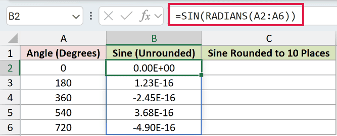
Below is the dataset. Column A lists zero and four multiples of 180 degrees.
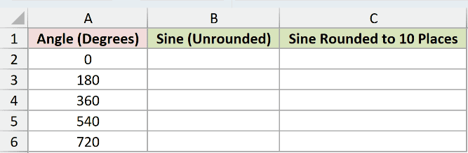
We want to inspect the raw sine results before rounding their tiny residues away.
Here is the unrounded formula:
=SIN(RADIANS(A2:A6))
And here is the formula that rounds those results to 10 decimal places:
=ROUND(B2:B6,10)
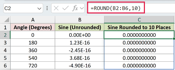
At 180 degrees, SIN returns roughly 1.23E-16, not zero. The residue reaches about -4.90E-16 at 720 degrees, with its sign alternating along the way.
This happens because Excel cannot store pi with perfect precision. The residue is tiny, but an exact comparison with zero can still fail.
ROUND makes every displayed result 0.0000000000. For comparison rules, you can also test whether the absolute result is smaller than a chosen tolerance.
Pro Tip: Do not turn on Excel’s Set precision as displayed option to remove these residues. That setting permanently changes stored values throughout the workbook.
Example 5: Convert Sine Back With ASIN
Finally, let’s reverse several sine values and see where that reversal has limits.
Below is the dataset. Column A lists angles from 15 through 150 degrees.
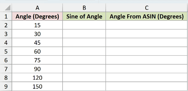
We want to calculate each sine, then use ASIN to return an angle in degrees.
Here is the formula that calculates the sine values:
=SIN(RADIANS(A2:A9))
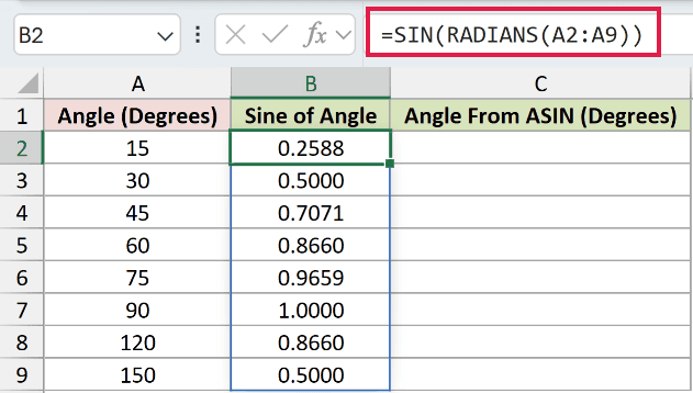
And here is the formula that converts those sine values back to angles:
=DEGREES(ASIN(B2:B9))
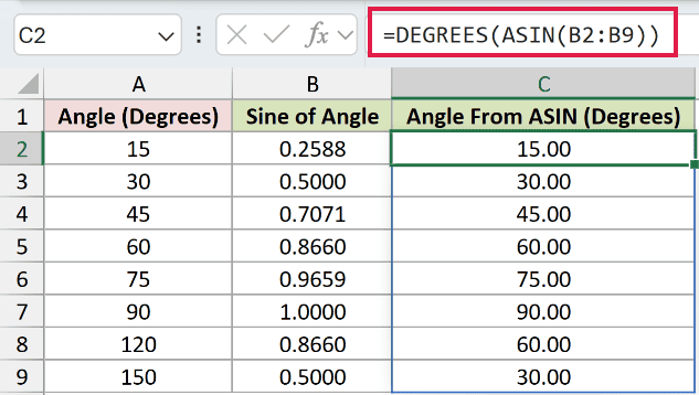
The 120 and 150 degree rows come back as 60.00 and 30.00. Those results are correct, not signs of a broken formula.
ASIN returns only its principal angle from -90 to 90 degrees. Sine is symmetric around 90 degrees, so ASIN cannot distinguish 120 from 60 or 150 from 30.
DEGREES converts ASIN’s radian result into degrees. When you need a full angle from two side measurements, ATAN2 is usually the better choice.
Tips & Common Mistakes
- SIN expects radians. Use RADIANS for degree inputs, or multiply the degrees by PI and divide by 180.
- SIN always returns a value from -1 to 1. Negative angles and angles beyond 180 degrees are valid.
- A blank reference is treated as zero, which can hide missing values in an angle column. Check for blanks when gaps matter.
- In Excel 2021 and later, range-based SIN formulas spill. If Excel inserts the implicit intersection operator, the formula returns one result instead.
- In Excel 2019 and earlier, enter the formula for the first angle and fill it down, or use the older array-entry method.
- Cell formatting changes the displayed decimals, not SIN’s stored result. Use ROUND when later calculations need a controlled precision.
- No newer Excel function replaces SIN. RADIANS, ASIN, COS, TAN, and ATAN2 solve related parts of trigonometric calculations.
SIN is straightforward once the input unit is right. Convert degrees to radians first, then use the result for measurements and related trigonometric work.
Keep the tiny residues near expected zeros in mind, and remember that ASIN returns only its principal angle.
Related Excel Functions / Articles:
