
The SINH function in Excel returns the hyperbolic sine of a number. It appears in calculations for hanging cables, where you need the curved length or slope along a span.
Its input is a plain number, not an angle. Negative inputs produce negative results, and positive inputs produce positive results that grow rapidly as the input increases.
I’ll show you how to calculate SINH for a list, work out cable lengths and slopes, and recover the original inputs from the results.
SINH Function Syntax in Excel
The SINH function takes a required number argument:
=SINH(number)
- number (required): The real number whose hyperbolic sine you want. You can supply a number, cell reference, or calculation.
SINH is available in every version of Excel. You don’t need to convert its input from degrees to radians.
When to Use SINH Function
- Calculate hyperbolic sine values for a list of model inputs.
- Find the curved length of a hanging cable when its span and catenary constant are known.
- Calculate how steeply a cable slopes at different positions along its span.
- Check a hyperbolic calculation against its exponential definition or reverse the calculation to recover an input.
Example 1: Calculate SINH for a List
Let’s start with a list that includes negative numbers, zero, and positive numbers.
Below is the dataset. Column A contains the inputs, and column B has the SINH Result header with cells ready for the answers.
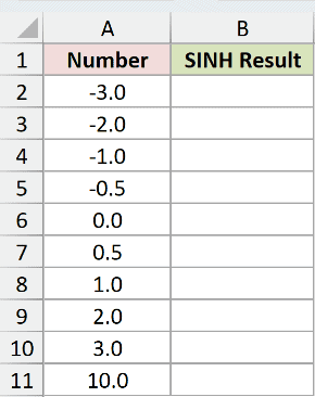
We want to calculate the hyperbolic sine of every number in column A.
Enter this formula in B2:
=SINH(A2:A11)
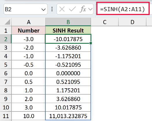
The formula spills into B2:B11, returning a separate answer for each input. You enter it only in the top cell.
This spilling version works in Excel 2021, Excel 2024, and Microsoft 365. In Excel 2019 and earlier, use a single-cell input and copy the per-row formula down.
The input -1.0 returns -1.175201, while 1.0 returns 1.175201. The magnitude stays the same when you reverse the sign.
At 0.0, the result displays 0.000000. But at 10.0, it reaches 11,013.232875, so the results can become large quickly.
Example 2: Calculate Hanging Cable Length
A hanging cable follows a curve called a catenary, so its length exceeds the horizontal distance between its supports.
Below is the dataset. Columns A:C list cable runs, span lengths, and catenary constants. Columns D:E are reserved for cable length and extra cable.
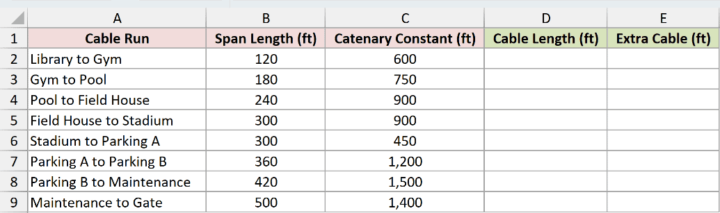
We want the curved cable length and the extra length beyond each horizontal span, assuming the supports are at the same height.
The catenary constant is horizontal tension divided by cable weight per foot. It’s a length in feet, so it uses the same units as the span.
Enter the cable-length formula in D2:
=2*C2:C9*SINH(B2:B9/(2*C2:C9))
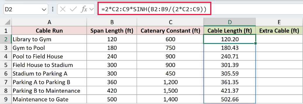
How this formula works:
B2:B9contains each horizontal span, andC2:C9contains its catenary constant.- The division inside SINH expresses half the span relative to the catenary constant.
- Multiplying the SINH result by twice the constant returns the full cable length in feet.
The results spill into D2:D9. Library to Gym needs 120.20 feet of cable across its 120-foot span.
Next, enter this formula in E2 to calculate the extra cable beyond each span:
=D2:D9-B2:B9
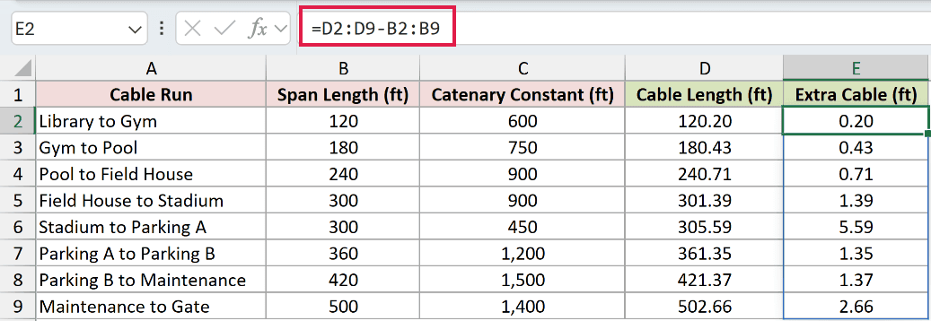
The formula subtracts each horizontal span from its curved cable length and spills into E2:E9. Library to Gym has 0.20 feet of extra cable.
Compare Field House to Stadium with Stadium to Parking A. Both spans are 300 feet, but their catenary constants are 900 and 450 feet.
The corresponding extra lengths are 1.39 and 5.59 feet. A smaller constant produces a more deeply hanging curve, so the same span needs more cable.
Example 3: Find Cable Slope Along a Span
Now let’s see how the cable’s slope changes as you move from the left pole to the right pole.
Below is the dataset. Column A lists positions; columns B:C will hold slope and angle. The Setting card contains the span length and catenary constant.
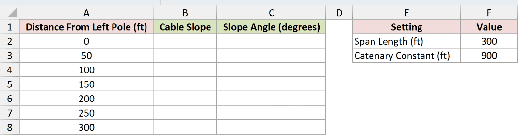
We want the slope at each position, followed by its angle relative to the horizontal.
The card contains typed inputs: 300 feet in F2 for the span and 900 feet in F3 for the catenary constant.
Enter this formula in B2:
=SINH((A2:A8-$F$2/2)/$F$3)
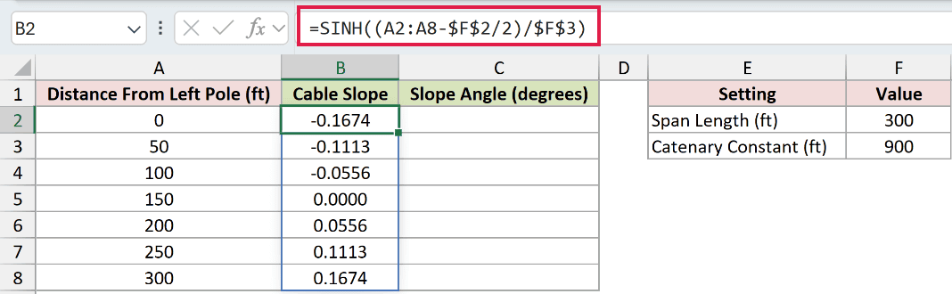
The formula subtracts half the span from each position, placing the origin at midspan. It then divides by the fixed catenary constant before applying SINH.
The slope spills into B2:B8. It measures vertical change relative to horizontal change, with the sign showing whether the cable falls or rises toward the right.
At the left pole, the slope is -0.1674. At the midpoint, 150 feet along, it’s 0.0000. At the right pole, it’s 0.1674.
To turn these slopes into angles, ATAN converts a slope to an angle in radians. DEGREES then converts that angle into degrees.
Enter the angle formula in C2:
=DEGREES(ATAN(B2:B8))
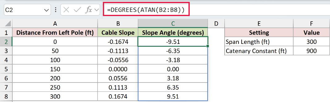
The angles spill into C2:C8. The endpoint angles display -9.51 and 9.51 degrees, while the midpoint displays 0.00 degrees.
SINH’s input remains a distance ratio throughout. The angle conversion happens afterward because we’re expressing the calculated slope as an angle.
Example 4: Check the Hyperbolic Relationships
You can check SINH against its exponential definition and then use it in a related hyperbolic ratio.
Below is the dataset. Column A contains test numbers, column B is reserved for SINH, and columns C:E provide space for the comparison calculations.
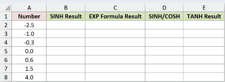
We want to compare SINH with its expanded definition, then check the ratio of hyperbolic sine to hyperbolic cosine.
Start with the SINH formula in B2:
=SINH(A2:A8)
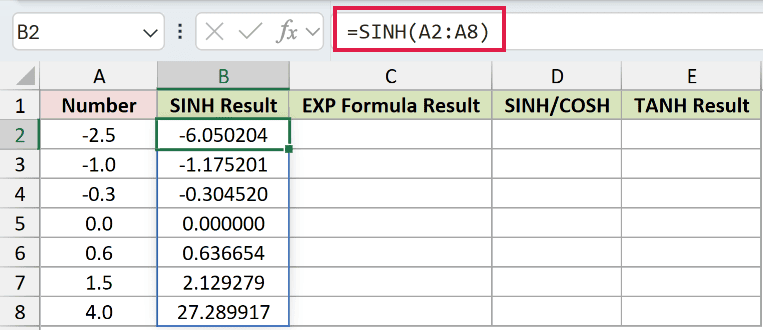
The results spill into B2:B8. For the input -2.5, SINH returns -6.050204.
EXP raises the mathematical constant e to a specified power. It lets us build SINH’s definition by subtracting the negative-input exponential from the positive-input exponential, then halving.
Enter this comparison formula in C2:
=(EXP(A2:A8)-EXP(-A2:A8))/2
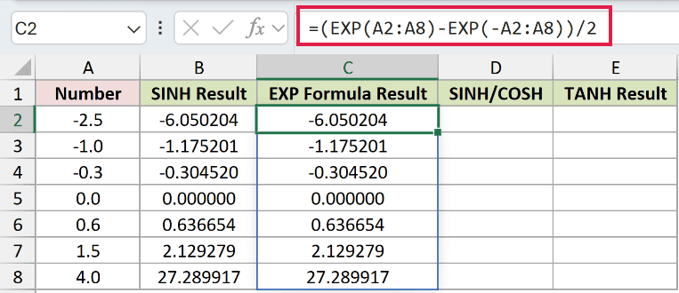
The comparison column spills into C2:C8 and matches the displayed SINH results. For -2.5, the expanded formula also returns -6.050204.
For the next comparison, COSH returns the hyperbolic cosine of each input. Dividing SINH by this value produces the hyperbolic tangent.
Enter this ratio formula in D2:
=SINH(A2:A8)/COSH(A2:A8)
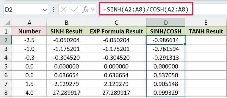
The comparison ratio spills into D2:D8. At -2.5, it displays -0.986614.
TANH calculates hyperbolic tangent directly, so it provides a check on the SINH-based ratio. Enter this comparison formula in E2:
=TANH(A2:A8)
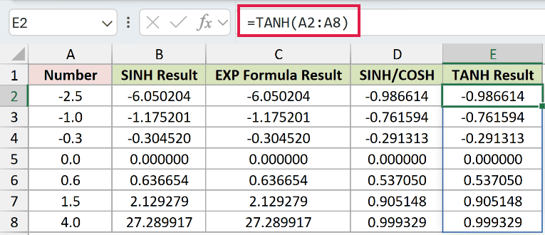
This comparison spills into E2:E8. Its -0.986614 result matches the ratio for -2.5, and the displayed results agree throughout these comparison columns.
Column C checks SINH itself, while columns D:E compare two ways of calculating hyperbolic tangent.
Example 5: Recover the Original Number
You can also reverse a SINH calculation to check that it leads back to the starting value.
Below is the dataset. Column A contains the original numbers, column B will hold SINH results, and column C is reserved for the reverse-calculation check.
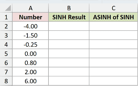
We want to calculate SINH and then recover each original number, including its sign.
Enter the SINH formula in B2:
=SINH(A2:A8)
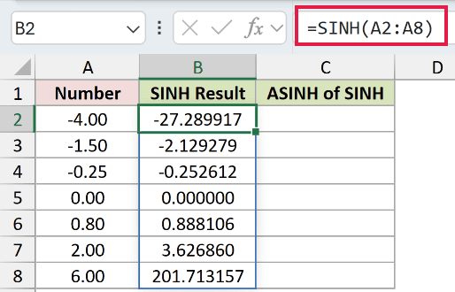
The results spill into B2:B8. The input -4.00 returns -27.289917, while 6.00 returns 201.713157.
ASINH returns the inverse hyperbolic sine. It reverses SINH, so we can use the calculated results to check the original inputs.
Enter this reverse-check formula in C2:
=ASINH(B2:B8)
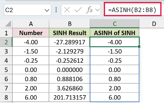
The check spills into C2:C8, recovering the original numbers. The results include -4.00 and 6.00, with the negative sign preserved.
Reference the calculated cells directly for this check. Retyping their displayed values would use rounded inputs instead of the values stored in the workbook.
Tips & Common Mistakes
- Don’t treat the input as an angle. SINH takes a plain number. Converting a model’s input from degrees to radians changes the calculation unnecessarily.
- Watch for numeric overflow. In testing, an input of
709worked, while710,711, and-711returned#NUM!. Very large inputs can exceed Excel’s calculation limits. - Check unexpected blanks. SINH treats a blank referenced cell as zero. A missing input can therefore look like a valid zero result.
- Text isn’t always rejected. Numbers stored as text can be converted, while nonnumeric text such as
abcreturns#VALUE!. TRUE is treated as the numeric input1. - Keep output cells clear. A blocked spill range causes
#SPILL!. Enter each range formula in its top result cell and leave room for the remaining results. - Keep cable units consistent. The span and catenary constant must use the same length unit. The constant is a length derived from tension and weight per unit length, not raw tension.
Related Excel Functions / Articles:
