
Excel’s TIMEVALUE function converts a time stored as text into a numeric Excel time value.
You can use the result in time calculations, such as finding hours between imported timestamps. Apply a time format when you want to display it as a clock time.
TIMEVALUE extracts the time portion. A date included in the text does not become part of the returned value.
In this article, I’ll show you how to convert text times, calculate hours between them, and combine separate text dates and times.
TIMEVALUE Function Syntax in Excel
The TIMEVALUE function takes one argument:
=TIMEVALUE(time_text)
- time_text (required) is text that Excel recognizes as a time. You can supply quoted text, a cell reference, or a range of text times.
Excel stores a time as a fraction of a day. TIMEVALUE returns that fraction, which you can display as a decimal or format as a clock time.
The input can include a date, but TIMEVALUE discards that part. We’ll look at what this means in Example 2.
When to Use TIMEVALUE Function
- Convert a pasted or imported column of text times into numeric time values.
- Keep only the clock time from text containing both a date and a time.
- Calculate elapsed hours between opening and closing times stored as text.
- Combine separate text date and time columns into one timestamp.
- Total short text durations or compare text clock-ins against a cutoff.
Example 1: Convert Text Times to Time Values
Let’s start with call times pasted into a worksheet as text.
Below is the dataset. Column A contains eight call IDs, and column B contains their start times stored as text.
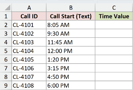
We want to convert all eight start times and see the numeric values Excel uses for calculations.
Here is the formula to enter in C2:
=TIMEVALUE(B2:B9)
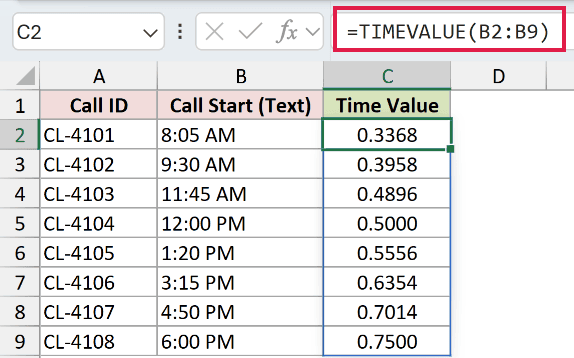
The formula spills into C2:C9. There’s no need to copy it down in Excel 2021 and later.
Column C uses the number format 0.0000, so 8:05 AM displays as 0.3368. That’s a fraction of a day, not decimal hours.
The noon entry displays as 0.5000, because noon is halfway through the day. The 6:00 PM entry displays as 0.7500.
Those decimals are useful for understanding the result. Apply a time format such as h:mm AM/PM when you want to read them as clock times.
Pro Tip: Adding zero is another way to convert recognizable text times, and it also accepts existing numeric times. TIMEVALUE is useful when your input is specifically text; check the input type if it returns #VALUE!.
Example 2: Extract Time From a Text Timestamp
Now let’s see what happens when the text includes a date too.
Below is the dataset. Column A lists building access points, and column B contains date-and-time entries stored as text.
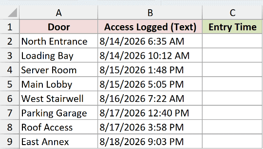
We want to extract each entry’s clock time and leave out its date.
Here is the formula to enter in C2:
=TIMEVALUE(B2:B9)
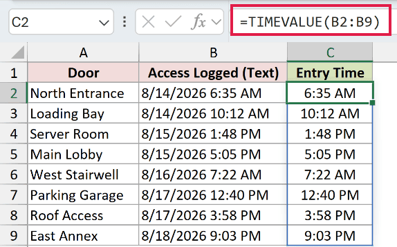
The formula spills into C2:C9, which uses the format h:mm AM/PM.
For North Entrance, 8/14/2026 6:35 AM becomes 6:35 AM. For East Annex, 8/18/2026 9:03 PM becomes 9:03 PM.
The date hasn’t been hidden by formatting. TIMEVALUE has removed it from the result, so changing the number format won’t bring the original date back.
VALUE returns both the date and time from the same text timestamp. Use it when you need both parts.
TIMEVALUE fits this example because we only want the clock time.
Pro Tip: These source timestamps use month/day/year order. Excel must recognize the text under your regional settings before TIMEVALUE can extract its time, even though the result discards the date.
Example 3: Calculate Hours Between Two Text Times
Let’s use the converted values in a calculation.
Below is the dataset. Column A lists help-desk tickets, while columns B and C contain their opening and closing times as text.
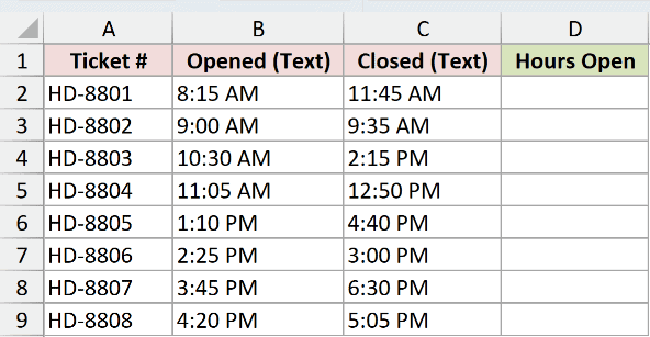
We want to calculate how many decimal hours each ticket stayed open on the same day.
Here is the formula to enter in D2:
=(TIMEVALUE(C2:C9)-TIMEVALUE(B2:B9))*24
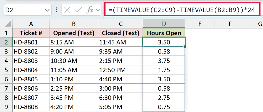
How this formula works:
- The first TIMEVALUE converts the closing times in
C2:C9. - The second TIMEVALUE converts the opening times in
B2:B9. - Subtracting gives the elapsed fraction of a day. Multiplying by
24converts that fraction to hours.
The results spill into D2:D9. Ticket HD-8801 runs from 8:15 AM to 11:45 AM, and its result displays as 3.50.
Ticket HD-8802 displays 0.58, while HD-8803 displays 3.75. Column D uses 0.00, so these are decimal hours rounded for display.
If your opening and closing cells already contain numeric times, you can subtract them directly. TIMEVALUE is needed here because both input columns contain text.
Example 4: Combine Text Dates and Times
Some exports put the date and time in separate columns.
Below is the dataset. Column A lists shipments, column B contains scan dates as text, and column C contains scan times as text.
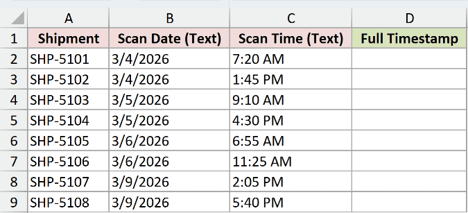
We want to combine each pair into one numeric timestamp that retains both the date and the time.
Here is the formula to enter in D2:
=DATEVALUE(B2:B9)+TIMEVALUE(C2:C9)
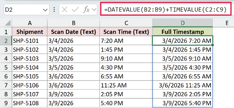
DATEVALUE converts the text dates into whole-number date values. TIMEVALUE converts the text times into fractions of a day, and adding them joins the two parts.
The results spill into D2:D9. With the format m/d/yyyy h:mm AM/PM, the first shipment displays as 3/4/2026 7:20 AM.
The last shipment displays as 3/9/2026 5:40 PM. These results retain their dates, unlike the clock-time-only results in Example 2.
Pro Tip: The dates in this example use month/day/year order. Confirm the source date order before converting an export, especially when both the month and day could be valid in either position.
Example 5: Total Text Durations With SUM
You can also convert text times inside a formula that returns one total.
Below is the dataset. Column A lists eight tasks, and column B contains time logged as text in hours:minutes form.
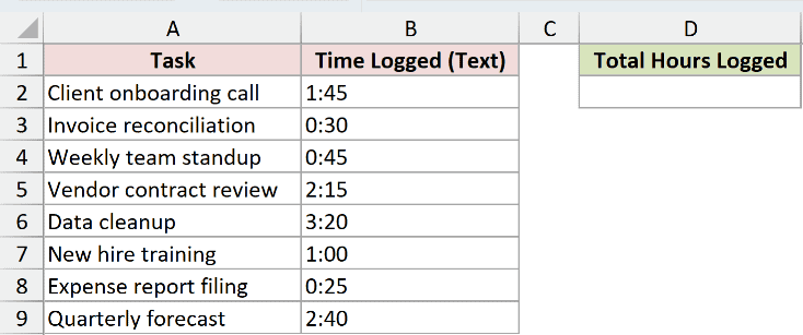
We want to total the logged durations and display the answer in decimal hours.
Here is the formula to enter in D2:
=SUM(TIMEVALUE(B2:B9))*24
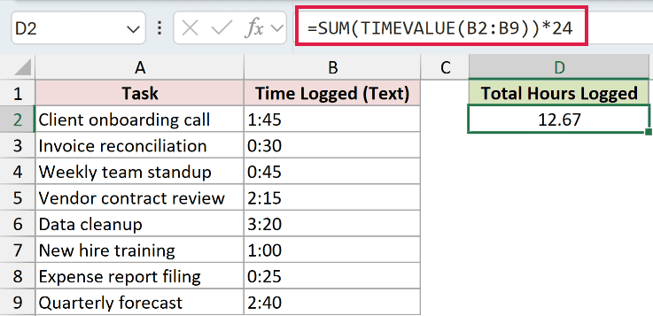
TIMEVALUE converts each text entry into a fraction of a day. SUM adds those fractions, and multiplying by 24 expresses the total in hours.
Cell D2 displays 12.67 using the number format 0.00. This is a rounded decimal-hours total, not hours and minutes separated by a decimal point.
Unlike the earlier examples, this formula doesn’t spill onto the worksheet. SUM combines the converted array into one answer.
Keep the result formatted as a number because the formula already converts it to hours. A clock-time format would misrepresent that number.
Pro Tip: This works because each duration is written as a valid clock-time string. TIMEVALUE is a clock-time parser, so don’t treat it as a general converter for individual durations of 24 hours or more.
Example 6: Flag Late Clock-Ins Against a Cutoff
Finally, let’s use TIMEVALUE to make a time comparison.
Below is the dataset. Column A contains employee names, and column B contains clock-in times stored as text.
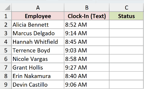
We want to flag clock-ins after 9:00 AM as Late and the remaining entries as On Time.
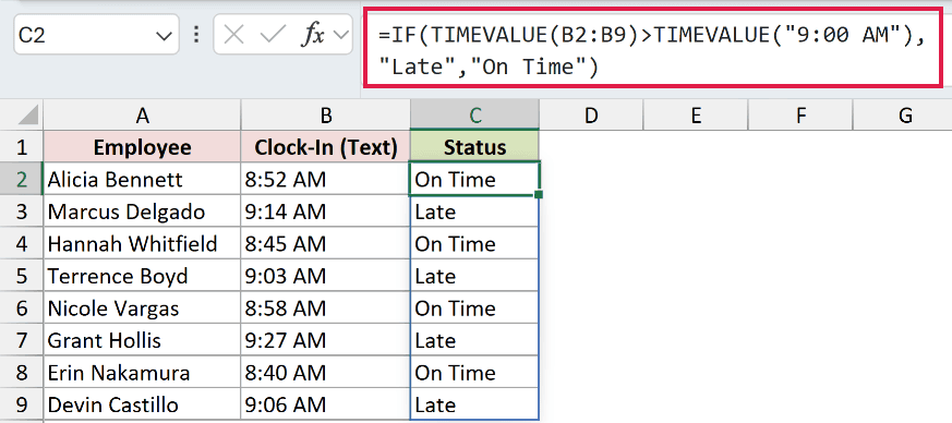
Here is the formula to enter in C2:
=IF(TIMEVALUE(B2:B9)>TIMEVALUE("9:00 AM"),"Late","On Time")
How this formula works:
- TIMEVALUE converts the text clock-ins in
B2:B9into numeric time values. - The second TIMEVALUE converts the quoted cutoff into the same kind of value.
- IF tests whether each clock-in is greater than the cutoff and returns the corresponding label.
The statuses spill into C2:C9. Alicia Bennett’s 8:52 AM entry returns On Time, while Marcus Delgado’s 9:14 AM entry returns Late.
Converting both sides means Excel compares actual times instead of text strings. The cutoff is entered directly in the formula, so there’s no separate cutoff cell.
Tips & Common Mistakes
- Check the input when you get
#VALUE!. TIMEVALUE expects text, so referencing a cell that already contains a numeric time returns this error. Numeric times need no conversion. Adding zero handles both numeric times and recognizable time text. Check for stray characters and regional separators when text fails. - Formatting doesn’t convert text. Applying a time format to the source column won’t make text numeric. Convert it first, then format the result for the way you want to read it.
- Allow room for spilled results. In Excel 2021 and later, blocked output cells cause
#SPILL!. An implicit-intersection@can reduce a range calculation to one result instead of the intended array. - Use the older array-entry method where needed. In Excel 2019 and earlier, select the full output range for a multi-result example and confirm the formula with Ctrl+Shift+Enter. For Example 5, select only the total cell before confirming.
- Watch for midnight crossings. Example 3 assumes both times fall on the same day. If a ticket closes after crossing midnight, its closing time is a smaller fraction of a day than its opening time. Subtracting gives negative hours. For an overnight interval shorter than a day, add a day to the closing time or wrap the difference with MOD. Longer intervals need full dates and times.
- Convert recurring exports during import. For a file you receive regularly, Power Query’s Time data type can handle the conversion as an import step instead of repeating worksheet cleanup.
Use TIMEVALUE when the source is text and you need the clock-time portion for a calculation.
If the date matters too, preserve it with VALUE or combine separate date and time inputs as shown in Example 4.
Other Excel articles you may also like:
