
Excel’s TRANSLATE function returns a translation of text using Microsoft’s translation service.
You can specify the source and target languages or let the service detect the source language. The function requires an internet connection and a supported Microsoft 365 version.
For customer-facing text, review the translation before using it. Names, abbreviations, and specialized terms can need extra context.
In this article, I’ll show you how to translate text into different languages, detect source languages automatically, and handle mixed-language reviews.
TRANSLATE Function Syntax in Excel
The TRANSLATE function accepts the text to translate, its source language, and the language you want back.
=TRANSLATE(text, [source_language], [target_language])
- text (required) is a quoted text string, cell reference, or range containing the text you want to translate.
- source_language (optional) is the source language code. If you omit it, Excel detects the language from the text. Microsoft’s language-code list shows the supported codes.
- target_language (optional) is the target language code. If you omit it, Excel uses your system language.
When to Use TRANSLATE Function
- Translate a column of labels, messages, or descriptions with one formula instead of sending each selection through the Translate pane.
- Convert mixed-language text into one common language.
- Create several language versions of the same phrase list.
- Pair TRANSLATE with DETECTLANGUAGE when you need visible, sortable source-language codes.
- Handle invalid language codes with a readable message instead of an Excel error.
Example 1: Translate App Text Into Spanish
Let’s start with a straightforward translation from English to Spanish.
Below is the dataset. Column A contains eight English app labels.
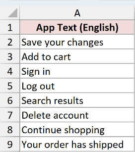
We want one formula to translate every label into Spanish.
Here is the formula:
=TRANSLATE(A2:A9,"en","es")
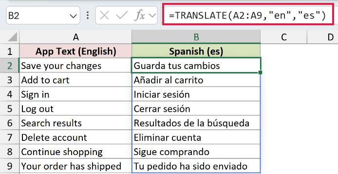
The range in the first argument makes the formula spill eight translations from B2 through B9.
The Spanish (es) header pairs the language name with its code. The en source code tells Excel the input is English.
When I calculated the workbook for this article, Microsoft’s service returned “Guarda tus cambios” for “Save your changes” and “Añadir al carrito” for “Add to cart”.
In that same calculation, the service returned “Sigue comprando” for “Continue shopping” and “Tu pedido ha sido enviado” for “Your order has shipped”.
Microsoft’s service can return different translations over time. These are the responses from this workbook’s calculation, and future results may differ.
Example 2: Detect the Source Language Automatically
Here’s a useful setup for a support inbox containing several languages.
Below is the dataset. Column A contains eight ticket subjects written in French, German, Spanish, Italian, Portuguese, Dutch, Swedish, and Polish.
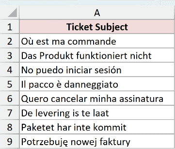
We want Excel to detect each source language and return every ticket subject in English.
Here is the formula:
=TRANSLATE(A2:A9,,"en")
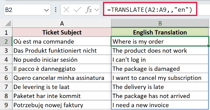
The double comma leaves source_language blank. Excel detects the language in each cell, while "en" fixes English as the target.
The workbook returned “Where is my order” and “The product does not work” first, and “I need a new invoice” last, when I calculated it for this article.
Pro Tip: Automatic detection suits a genuinely mixed column. When you already know the source language, pass its code because short text can be ambiguous.
Example 3: Detect and Translate Mixed-Language Reviews
Now let’s keep the detected language codes visible before translating the text.
Below is the dataset. Column A contains eight customer reviews in different languages.
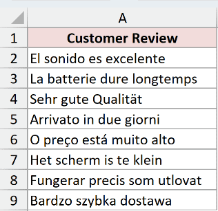
We first want to identify the language used in every review.
Here is the DETECTLANGUAGE formula:
=DETECTLANGUAGE(A2:A9)
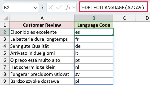
The service returned es, fr, de, it, pt, nl, sv, and pl in B2:B9 when I calculated this workbook for the article.
We can now feed those detected languages into TRANSLATE and return the reviews in English.
Here is the TRANSLATE formula:
=TRANSLATE(A2:A9,DETECTLANGUAGE(A2:A9),"en")
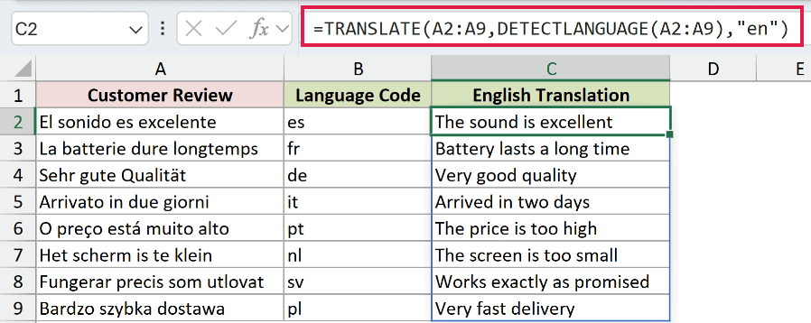
DETECTLANGUAGE supplies one source code for each review. TRANSLATE uses those codes with the matching text and spills the English results into column C.
At this article’s time of writing, the first three translations were “The sound is excellent,” “Battery lasts a long time,” and “Very good quality.”
Pro Tip: If the language codes already spill from B2, =TRANSLATE(A2:A9,B2#,"en") can point to that complete spill range.
Example 4: Translate One List Into Four Languages
Let’s turn one English phrase list into a four-language grid.
Below is the dataset. Column A contains seven storefront phrases, while B1:E1 contains the target codes es, fr, de, and it.
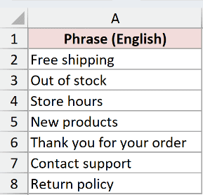
We want one formula to translate every phrase into Spanish, French, German, and Italian.
Here is the formula:
=TRANSLATE(A2:A8,"en",B1:E1)
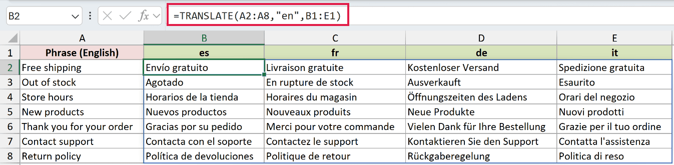
Excel combines the seven-row text range with the four-column code range. The result spills into a 7 by 4 grid from B2 through E8.
“Free shipping” returned “Envío gratuito,” “Livraison gratuite,” “Kostenloser Versand,” and “Spedizione gratuita” across the first output row when the workbook was calculated at the time of writing.
For “New products,” the service returned “Nuevos productos,” “Nouveaux produits,” “Neue Produkte,” and “Nuovi prodotti.”
Each code in the header controls one output column. You can change a code there without rewriting the formula.
Example 5: Handle Invalid Codes With IFERROR
Finally, let’s deal with a mistyped language code without hiding the source phrase inside the formula.
Below is the dataset. Column A lists six target codes, and E2 contains the phrase “Thank you.” The code xq is deliberately invalid.
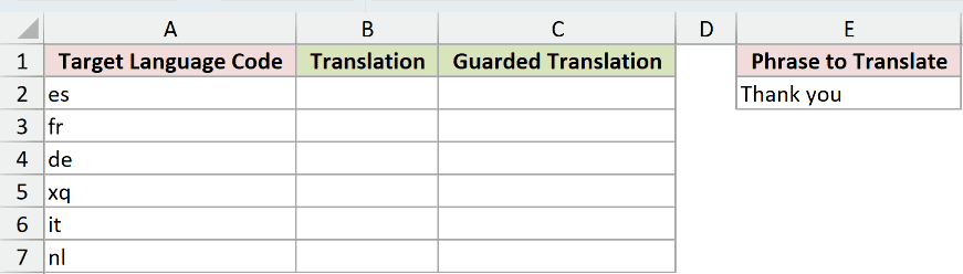
We first want to translate the phrase for each code and see the original error.
Enter this formula in B2 and copy it down through B7:
=TRANSLATE($E$2,"en",A2)
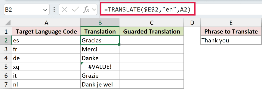
The absolute reference keeps the source phrase fixed while the target-code reference changes on each row.
At the time I prepared this article, the valid rows returned “Gracias,” “Merci,” “Danke,” “Grazie,” and “Dank je wel.” Cell B5 returned #VALUE! for xq.
Now we can replace that error with a clearer message.
Enter this formula in C2 and copy it down through C7:
=IFERROR(TRANSLATE($E$2,"en",A2),"Check this language code")
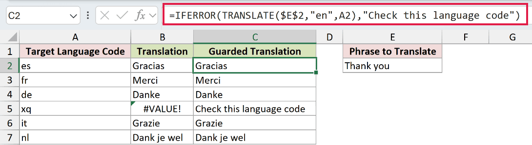
IFERROR returns “Check this language code” in C5 and leaves the valid translations unchanged. IFNA would not catch this problem because the error is #VALUE!.
This example stays per row so the bad code can be checked by itself. With valid codes, TRANSLATE can also spill this pattern from one formula.
Tips & Common Mistakes
#BUSY!means the service is still answering and may clear on its own.#CONNECT!usually means Excel cannot reach the service.#VALUE!can indicate an unsupported language code, a mistyped code, or non-text input.#NAME?means your Excel version does not include TRANSLATE.- Always supply
target_language. Otherwise, the result depends on the system language of the computer opening the workbook. - Supply
source_languagewhen you know it. Leave it blank only when Excel needs to detect mixed-language text. - A blocked output range causes
#SPILL!. Clear the cells where Excel needs to place the translated results. - Excel can return service errors when text is too long or the daily translation quota is reached.
- Treat each cell in a spill as a separate service request when watching the quota. Microsoft does not document the exact counting method.
- Machine translation is a useful first draft, but customer-facing or sensitive text still needs a human review.
TRANSLATE works best when you supply the language codes you know and leave source detection for mixed-language text.
Because the wording comes from a live service, check important translations before you publish or send them.
Related Excel Functions / Articles:
