If you want to combine two or more tables or ranges into one continuous list, the VSTACK function is the one you’re looking for.
VSTACK is a dynamic array function. It spills the combined result across the cells below, and it needs Microsoft 365 or Excel for the web.
In this article, I’ll walk you through five examples that cover the most common ways to use it.
VSTACK Function Syntax in Excel
The VSTACK function stacks multiple ranges or arrays on top of each other into one vertical list.
=VSTACK(array1, [array2], ...)
- array1 (required): The first range, table, or array you want to stack.
- array2, … (optional): Additional ranges to stack below array1, in the order you list them. You can include up to 253 arrays. If the input arrays have different numbers of columns, VSTACK pads the shorter rows with #N/A.
When to Use VSTACK Function
- Combine same-shape tables from multiple sheets or regions into one list.
- Append a new data range to an existing table in a single formula.
- Build one contiguous range to feed into SORT, UNIQUE, or FILTER functions.
- Replace the manual copy-paste routine when consolidating reports from different sources.
- Feed a combined range into a pivot table or structured summary.
Example 1: Stack Two Tables Into One List
Let’s start simple.
Below is a dataset with two separate sales tables sitting side by side. Columns A-C hold the Q1 results with a header row, and columns E-G hold the Q2 data rows.
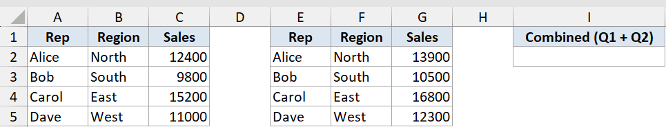
I want to combine both tables into one list, keeping the Q1 header and appending the Q2 data rows below it.
Here is the formula:
=VSTACK(A1:C5,E2:G5)
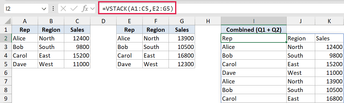
VSTACK takes the Q1 table (A1:C5, including the header) and stacks the Q2 data rows (E2:G5, no header) directly below it. The result is a single 9-row list that spills down from the formula cell automatically.
Change any value in the source tables and the combined list updates live without you touching the formula.
Pro Tip: Because VSTACK spills, make sure the cells below the formula are empty. If another cell is in the way, VSTACK returns a #SPILL! error until you clear the blocked range.
Example 2: Stack Three Ranges in One Formula
Here’s another practical scenario.
Below is a dataset with three small regional team lists sitting side by side in columns A-B, D-E, and G-H. Each list has its own header row.
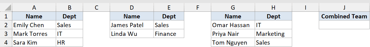
I want to merge all three teams into one combined list, keeping only the first header.
Here is the formula:
=VSTACK(A1:B4,D2:E3,G2:H4)
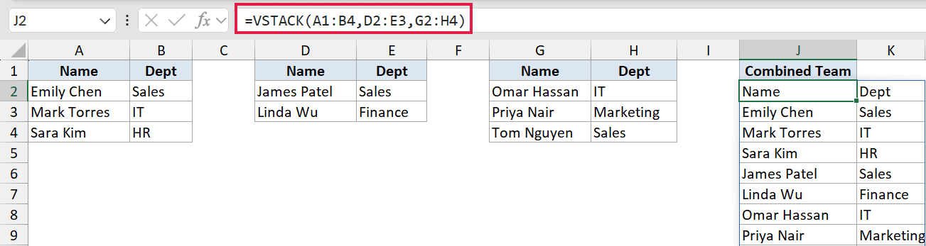
The first range (A1:B4) includes the header row. The second and third ranges (D2:E3 and G2:H4) start at row 2 to skip their headers. VSTACK lines them all up and spills the full list below the formula cell.
The formula barely gets longer no matter how many tables you add. Going from two to five is just a matter of tacking on more range arguments.
Example 3: Skip Duplicate Headers With DROP
Let’s step it up a bit.
Below is a dataset with two order tables. Columns A-C have the first batch, and columns E-G have the second batch. Both tables have a header row labeled “Order ID”, “Product”, and “Amount”.
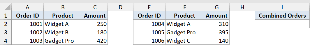
I want to stack both tables into one list, but without the second table’s header appearing in the middle of the combined results.
Here is the formula:
=VSTACK(A1:C4,DROP(E1:G4,1))
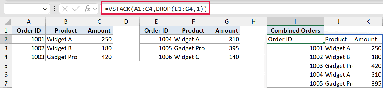
VSTACK(A1:C4) takes the first table with its header row intact. DROP(E1:G4, 1) removes the first row of the second table before VSTACK sees it, so the header never makes it into the combined list.
The final output is a single-header list with all the data rows from both tables.
Pro Tip: Without DROP, every table after the first brings its own header into the middle of the combined list. Wrap any extra range in DROP(range, 1) to strip its header row before stacking.
Example 4: Build a Sorted Master List (VSTACK + SORT)
Now let’s combine VSTACK with SORT.
Below is a dataset with two product price tables. Columns A-B have three products and columns D-E have four more. Both tables have data rows only (no header).
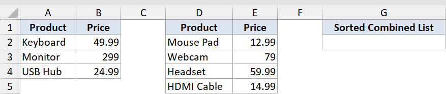
I want to merge both price tables into one list and sort everything A to Z by product name.
Here is the formula:
=SORT(VSTACK(A2:B4,D2:E5),1,1)
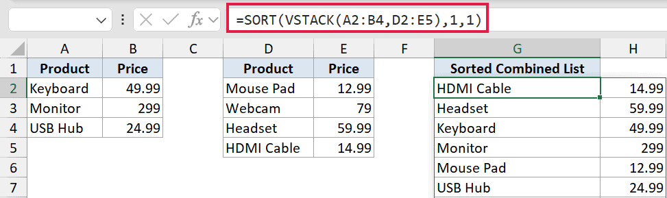
VSTACK(A2:B4, D2:E5) merges both price tables into one 7-row array. SORT then arranges that array by its first column in ascending order.
One thing to know: the sort index 1 refers to the first column of the stacked array, not a worksheet column letter. The whole thing spills as one sorted list.
Example 5: Merge and Deduplicate (VSTACK + UNIQUE)
Let’s finish with a useful combo.
Below is a dataset with two skill lists for separate teams. Column A holds Team A’s skills and column C holds Team B’s skills. Some skills appear in both lists.
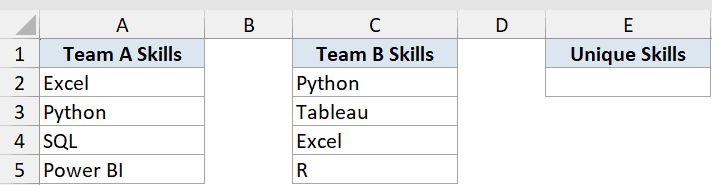
I want a single list of all the skills across both teams, with each skill appearing only once.
Here is the formula:
=UNIQUE(VSTACK(A2:A5,C2:C5))
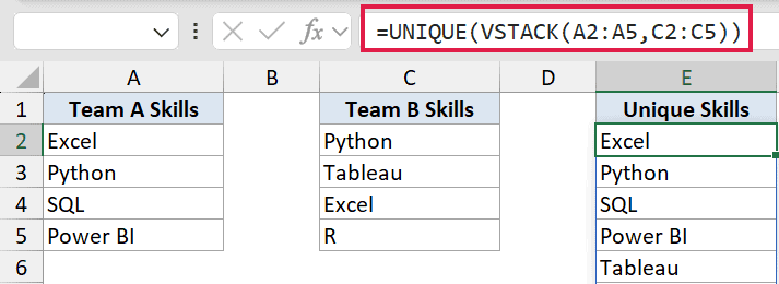
VSTACK(A2:A5, C2:C5) stacks both skill columns into one 8-item list, duplicates included. UNIQUE then strips those down, returning each skill just once.
Both Excel and Python appeared in both team lists and collapse to one entry each. The result spills as 6 unique skills.
Tips & Common Mistakes
- Different column counts pad with #N/A. If one array has 3 columns and another has 2, VSTACK pads the shorter row with #N/A. Wrap the result in IFNA to replace those with a blank or zero:
=IFNA(VSTACK(A1:C5, E1:F3), ""). - Empty source cells show as 0. Blank numeric cells in the source ranges appear as 0 in the stacked output, not as blanks. Keep that in mind if you’re summing or averaging the combined list.
- Needs Microsoft 365 or Excel for the web. VSTACK is not available in Excel 2019, 2021, or older versions. If you share the file with someone on an older version, the formula returns a #NAME? error.
- Use HSTACK to stack side by side. VSTACK stacks arrays vertically (more rows). If you need to add columns instead, use the HSTACK function, which stacks horizontally.
- Watch out for #SPILL! errors. VSTACK spills its output into the cells below. If any cell in the spill range is occupied, you’ll get a #SPILL! error. Clear the blocked cells to fix it.
VSTACK is one of those functions that earns its place fast. Once you stop copy-pasting ranges together and let a single formula handle the consolidation, you won’t want to go back.
Related Excel Functions / Articles: