
Excel’s EXPAND function enlarges an array to a specified number of rows and columns. It fills the added cells with a value you choose or with #N/A by default.
The row and column arguments set the final size of the result. They do not tell Excel how many rows or columns to add.
In this article, I’ll show you how to add rows and columns with padding, resize filtered results, and align arrays before combining them with HSTACK.
EXPAND Function Syntax in Excel
The EXPAND function uses the following syntax:
=EXPAND(array, rows, [columns], [pad_with])
arrayis the source range or array you want to enlarge.rowsis the total number of rows required. If omitted or left empty, Excel keeps the source array’s height.[columns]is the optional total number of columns required. If omitted, Excel keeps the source array’s width.[pad_with]is the optional value placed in added cells. If omitted, Excel returns#N/Ain those cells.
When to Use EXPAND Function
- Fit a small dataset into a fixed report area.
- Add blank or labeled rows and columns to an array.
- Give variable filtered results a consistent size.
- Align arrays of different heights before combining them.
- Calculate dimensions from the source. The ROWS function returns its height, while the COLUMNS function returns its width.
Example 1: Expand Rows With Text Padding
Let’s start by adding rows and using a clear text value for the padded cells.
Below is a delivery assignment dataset in A2:D5, with route, driver, zone, and vehicle type columns.

The finished schedule should have six rows and four columns, with every added cell displaying “Not scheduled.”
Here is the formula:
=EXPAND(A2:D5,6,4,"Not scheduled")
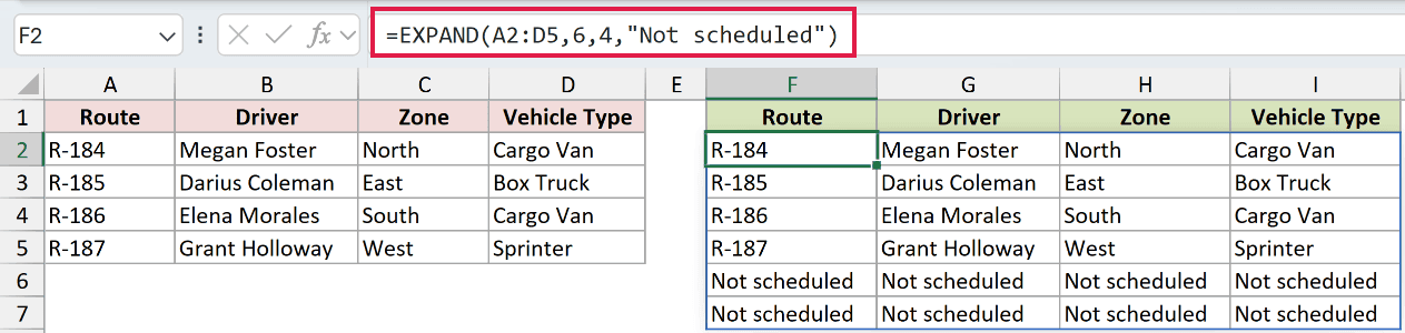
The source already has four rows and four columns. EXPAND keeps those values, then adds two rows to reach the requested six-row height.
The fourth argument fills all eight added cells with “Not scheduled.” The complete array spills from F2 through I7.
Pro Tip: The values 6 and 4 are the final dimensions. They do not mean “add six rows and four columns.”
Example 2: Add Blank Columns With EXPAND
You can enlarge only one dimension and leave the other unchanged.
Below is an inventory dataset in A2:C6 containing part numbers, descriptions, and quantities on hand.

The goal is to add blank Bin and Next Delivery columns while keeping all five inventory rows.
Here is the formula:
=EXPAND(A2:C6,,5,"")
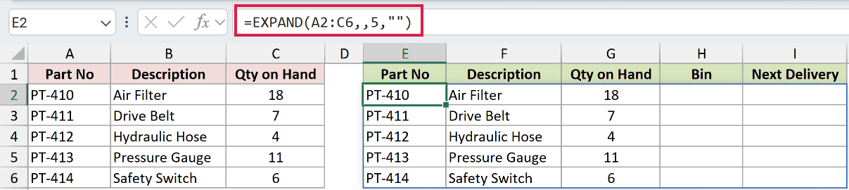
The empty second argument tells EXPAND to keep the source array’s five rows. The value 5 makes the result five columns wide.
The empty text string fills the new Bin and Next Delivery cells. The result spills across E2:I6.
Those blank-looking cells belong to the spill and cannot be edited individually. Use separate input columns if Bin and Next Delivery need manual entries.
Pro Tip: Empty text from "" looks blank, but some formulas treat it differently from a truly empty cell.
Example 3: Use the Default #N/A Padding
Leaving out the padding argument makes EXPAND’s default behavior easy to see.
Below is a volunteer registration dataset in A2:C5 containing names, events, and registration statuses.
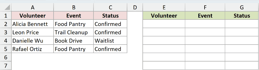
This list needs six rows without changing its three-column width.
Here is the formula:
=EXPAND(A2:C5,6)
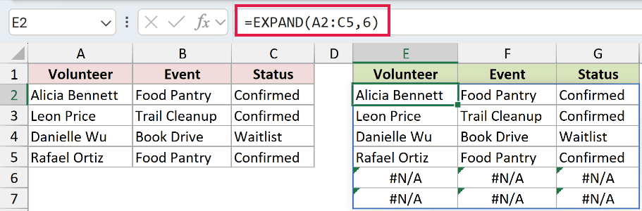
The source contains four rows, so EXPAND adds two more. Because the columns argument is omitted, the result stays three columns wide.
The formula also omits pad_with. Excel therefore places #N/A in each of the six added cells rather than treating the formula as broken.
Use "", zero, or a text label as the fourth argument when another value would make the output clearer.
Example 4: Expand FILTER Results to a Fixed Size
EXPAND can give a variable dynamic array a consistent footprint.
Below is a maintenance backlog in A2:D11, with ticket ID, asset, priority, and status columns.
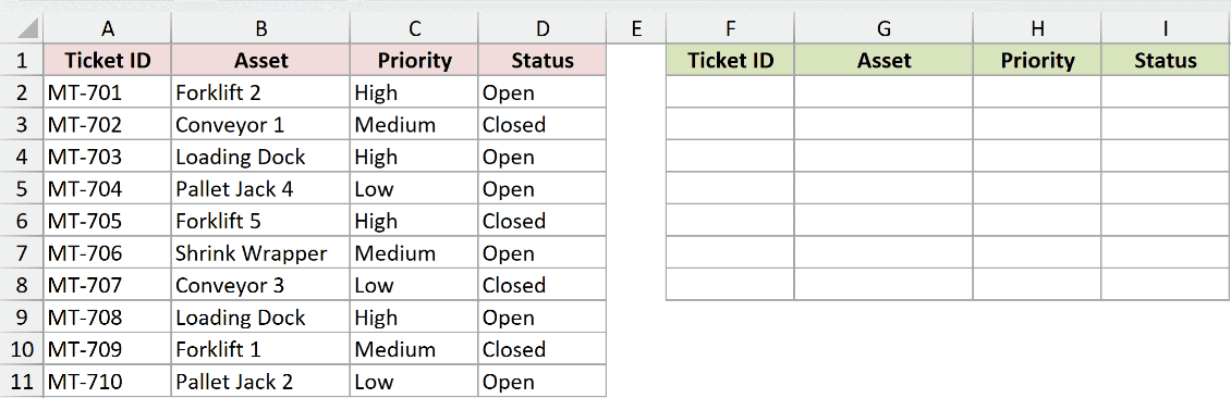
The report should return the open tickets in seven rows, leaving any unused row blank.
Here is the formula:
=EXPAND(FILTER(A2:D11,D2:D11="Open"),7,4,"")
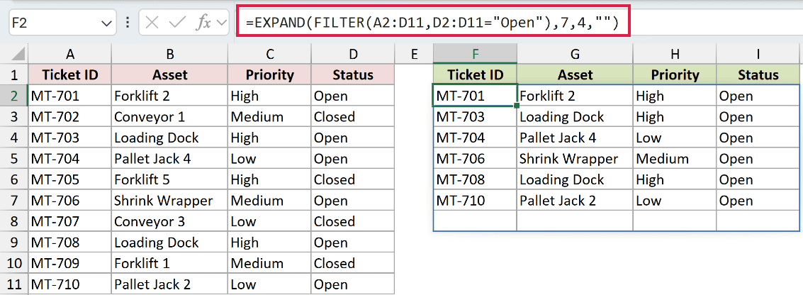
How this formula works:
FILTER(A2:D11,D2:D11="Open")returns the six records whose status is Open.- EXPAND sets that filtered array to seven rows and four columns.
- The empty text string fills the final unused report row.
If the filtered result grows beyond seven rows, EXPAND returns #VALUE! because it cannot shrink the array to the requested size.
Pro Tip: EXPAND shapes the result returned by FILTER. It does not limit the number of matching records, so choose a target large enough for the expected result.
Example 5: Align Arrays Before Using HSTACK
Padding a shorter array can keep side-by-side reports aligned.
Below are six weeks of forecast sales in A2:B7 and four weeks of actual sales in D2:E5.
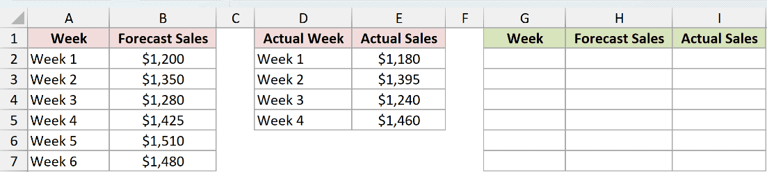
The final report needs six rows, with the forecast and actual sales placed beside the same weeks.
Here is the formula:
=HSTACK(A2:B7,EXPAND(E2:E5,6,1,""))
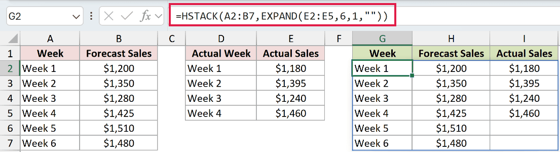
How this formula works:
EXPAND(E2:E5,6,1,"")extends the four actual sales values to six rows and fills the last two positions with empty text.- The HSTACK function places the six-row forecast array beside the padded actual sales array.
- The result keeps Week 1 through Week 6 aligned, with blanks where actual sales are unavailable.
Pro Tip: This setup assumes the actual sales are already in the same chronological order as the forecast weeks. EXPAND changes the size, not the order.
Example 6: Add Rows With a Calculated Target
A calculated row argument is useful when the result should be larger than the source by a fixed amount.
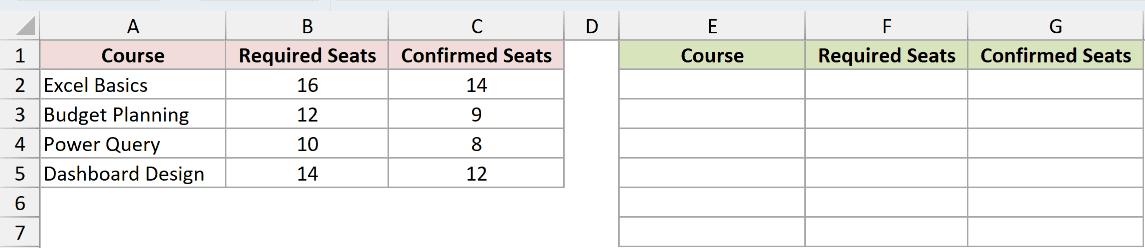
Below is a training plan in A2:C5, with course names, required seats, and confirmed seats.
The training plan needs two buffer rows, with every added cell filled with zero.
Here is the formula:
=EXPAND(A2:C5,ROWS(A2:C5)+2,,0)
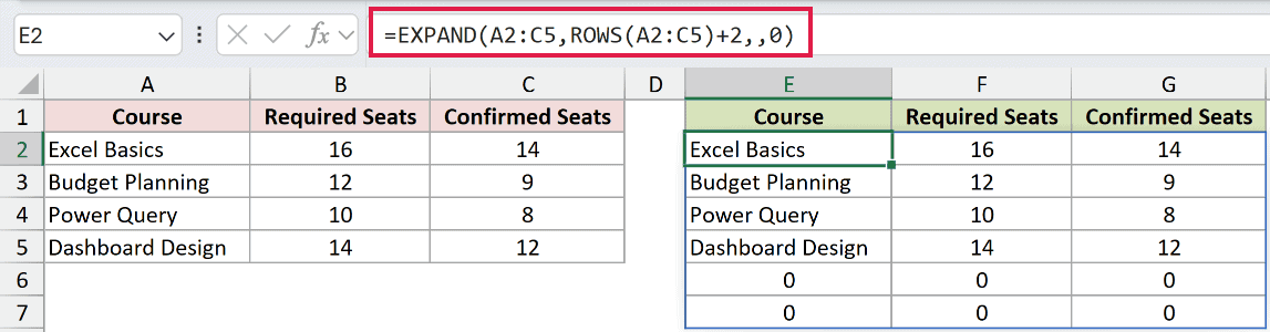
ROWS counts the four records in A2:C5, and adding 2 sets the target height to six rows. The omitted columns argument preserves the three-column width.
The final argument fills both added rows with zeros. The result spills from E2 through G7.
Pro Tip: The reference A2:C5 is fixed. If your source will grow, use an Excel Table or another reference that expands with the data.
Tips & Common Mistakes
- EXPAND is available in Microsoft 365 and Excel 2024 for Windows and Mac. Excel 2021 and earlier do not support it.
- Keep the spill area clear. Any value blocking the returned array causes a
#SPILL!error. rowsandcolumnsspecify the final dimensions. Asking for fewer rows or columns than the source contains returns#VALUE!.- An output that exceeds Excel’s array limits returns
#NUM!. - Omitting
pad_withproduces#N/Ain every added cell. Supply"", zero, or text when that default does not suit the report. - Enter the formula outside an Excel Table because spilled array formulas cannot expand inside a table.
- EXPAND changes an array’s dimensions without sorting, filtering, or moving its existing values.
I covered how to expand either dimension, control padding, shape filtered results, align arrays, and calculate a target size.
I hope you found this article helpful.
Related Excel Functions / Articles:
