If you want to test whether an odd number of conditions are true (and only then return TRUE), the XOR function in Excel is what you’re after.
It’s the exclusive OR, and it behaves a little differently from the regular OR you might be used to.
In this article, I’ll walk you through how XOR works, the truth table, the syntax, and a few practical examples you can drop into your own sheets.
XOR Function Syntax
Here is the syntax of the XOR function:
=XOR(logical1, [logical2], ...)
- logical1 – The first condition or value you want to test. Required.
- logical2, … – Additional conditions or values. Optional. You can pass up to 254 more arguments, so 255 total.
Each argument can be a logical value (TRUE / FALSE), a number (zero counts as FALSE, anything else counts as TRUE), or a cell reference/range that evaluates to either.
Quick Refresher: What Exclusive OR Means
Plain OR returns TRUE if at least one argument is TRUE.
XOR is stricter.
With two arguments, XOR returns TRUE only when exactly one of them is TRUE, not both.
Here’s the two-argument truth table:
| A | B | A OR B | A XOR B |
|---|---|---|---|
| TRUE | TRUE | TRUE | FALSE |
| TRUE | FALSE | TRUE | TRUE |
| FALSE | TRUE | TRUE | TRUE |
| FALSE | FALSE | FALSE | FALSE |
The row that matters is the first one. OR says “yes, at least one is TRUE”, but XOR says “no, they’re both TRUE, so it’s not exclusive anymore”.
The Key Rule for 3 or More Arguments
This trips a lot of people up.
With three or more arguments, XOR does NOT mean “exactly one TRUE”. It means “an ODD number of TRUEs”.
So:
- 1 TRUE out of 3 args → result is TRUE (odd)
- 2 TRUEs out of 3 args → result is FALSE (even)
- 3 TRUEs out of 3 args → result is TRUE (odd)
- 0 TRUEs → result is FALSE (zero is even)
If you actually need “exactly one TRUE” across many arguments, XOR won’t give it to you on its own.
You’d need something like =COUNTIF(range, TRUE)=1 instead.
Worth keeping in mind.
When to Use XOR
Use this function when you need to:
- Test if exactly one of two conditions is met (classic exclusive choice)
- Check whether an odd number of TRUE values exists in a list
- Build a toggle that flips state when one input changes
- Catch records that meet one criterion but not the other
Let me show you a few practical examples.
Example 1: Either Discount, Not Both
Let’s start with a simple example.
Say you have a list of orders, and a customer qualifies for a discount if they’re either a member OR have placed a bulk order, but not both at the same time (because that would stack discounts, which the policy doesn’t allow).
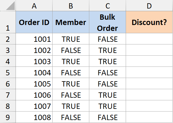
Below is the dataset. Column A has the order ID, column B says whether the customer is a member (TRUE / FALSE), and column C says whether the order is a bulk order.
Here is the formula:
=XOR(B2, C2)
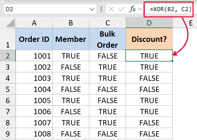
In the above formula, XOR returns TRUE only when exactly one of the two columns is TRUE. If the customer is both a member and has placed a bulk order, the formula returns FALSE, because the policy doesn’t allow stacking.
This is the cleanest use case for XOR, and it reads almost like English: “one or the other, but not both”.
If you’re using a newer version of Excel, you would have access to dynamic arrays, and you can also use the formula below.
=BYROW(B2:C9,XOR)
TIBA formula also does the same thing, but instead of you applying the formula for one row and then copying it down, it takes up the entire array, which is B2 to C9, and applies the XOR function to each row.
Example 2: Wrap XOR Inside IF for a Readable Result
The TRUE / FALSE output is fine, but you usually want something nicer in the cell.
Now let’s look at something a bit more readable. Same dataset as Example 1, but I’ll wrap XOR inside an IF function to print “Apply Discount” or “No Discount”.
Here is the formula:
=IF(XOR(B2, C2), "Apply Discount", "No Discount")
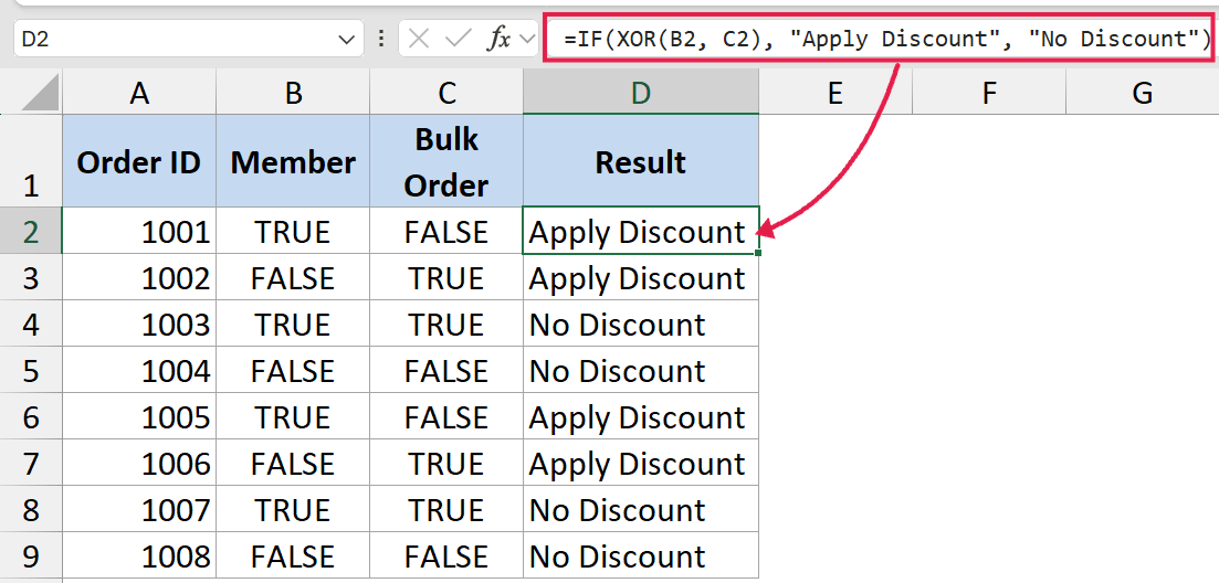
Here, the XOR part does the logic, and IF turns the result into a label. If exactly one of B2 or C2 is TRUE, you get “Apply Discount”. If both or neither, you get “No Discount”.
You can swap the two text labels for anything you need. The same pattern works for “Pass / Fail”, “Eligible / Not Eligible”, and so on.
Example 3: Parity Check Across Multiple Columns
Here’s a more interesting one.
You have five quality-control checks per item, and an item should be flagged for manual review if an odd number of checks failed.
An even number of failures means the system can route it automatically (whether all clean or grouped flags it can handle).
I know that sounds like a contrived rule, but parity checks like this come up often in error detection (think barcodes, ISBNs, networking). XOR handles it natively.
Below I have a data set where I want to check the true and false values in each row and only highlight if there is an odd number of TRUES.

Here is the formula:
=XOR(B2:F2)
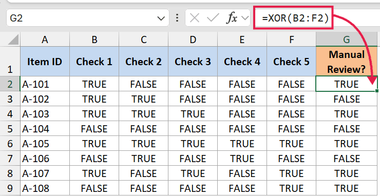
XOR walks through every TRUE in the range B2:F2 and returns TRUE if the count is odd, FALSE if even. No need to count anything yourself.
If you need to convert that to a label, wrap it in IF the same way as Example 2.
Pro Tip: XOR ignores text and empty cells when you pass a range. So if a check cell is blank or contains text like “N/A”, it won’t affect the parity count. Only TRUE / FALSE and numeric values are counted.
Example 4: XOR vs AND vs OR vs NOT
People sometimes reach for XOR when they actually want AND, OR, or NOT. Quick comparison so you don’t mix them up.
| Function | Returns TRUE when… |
|---|---|
| AND | All arguments are TRUE |
| OR | At least one argument is TRUE |
| NOT | The single argument is FALSE (it just flips it) |
| XOR | An odd number of arguments are TRUE |
Same two inputs A and B:
| A | B | AND | OR | XOR |
|---|---|---|---|---|
| TRUE | TRUE | TRUE | TRUE | FALSE |
| TRUE | FALSE | FALSE | TRUE | TRUE |
| FALSE | TRUE | FALSE | TRUE | TRUE |
| FALSE | FALSE | FALSE | FALSE | FALSE |
The only row where OR and XOR disagree is the top one. That’s the whole point of XOR.
If your real-world rule is “at least one but not all”, XOR alone won’t do it past two arguments. You’d combine OR with NOT(AND(…)) instead. Something like =AND(OR(A,B,C), NOT(AND(A,B,C))).
Tips & Common Mistakes
- Don’t confuse “odd number of TRUEs” with “exactly one TRUE”. With two arguments these are the same thing. With three or more they aren’t. If your business rule is literally “exactly one”, use COUNTIF instead of XOR.
- XOR ignores text and blanks in a range. That’s usually helpful, but if you expect every cell to be evaluated and one is blank, your result might surprise you. Convert text flags to TRUE / FALSE first if you need them counted.
- Numbers count as logical values. Zero is FALSE, any non-zero number is TRUE. So
=XOR(0, 5, 0)returns TRUE because there’s one non-zero (odd count). - #VALUE! error shows up when an argument is text that can’t be evaluated as a logical or number. For example,
=XOR(B2, "yes")returns #VALUE!. - XOR is available from Excel 2013 onwards. If you’re on an older version, build it from AND / OR / NOT instead.
XOR isn’t a function I reach for every day, but when the rule is “one or the other, not both” or “odd number of these conditions are true”, it saves a surprising amount of formula writing. The two-argument case is the easy one. Just remember the parity rule for three or more, and you’re set.
Related Excel Functions / Articles:
- Using Conditional Formatting with OR Criteria in Excel
- ‘Does Not Equal’ Operator in Excel (Examples)
- How to Use Greater Than or Equal to Operator in Excel Formula?
- How to Compare Two Cells in Excel? (Exact/Partial Match)
- Microsoft Excel Terminology (Glossary)
- Using IF Function with Dates in Excel (Easy Examples)
- SUMPRODUCT vs SUMIFS Function in Excel
- How to use Excel If Statement with Multiple Conditions Range [AND/OR]