
The Z.TEST function in Excel returns the upper-tail p-value for a one-sample z-test.
It helps you judge whether a sample mean is significantly higher than a benchmark. Excel can use a known population standard deviation or estimate it from the sample.
In this article, I’ll show you how to choose the correct tail, report a complete test result, and test several benchmarks at once.
Z.TEST Function Syntax in Excel
The Z.TEST function takes a sample, a hypothesized population mean, and an optional known population standard deviation.
=Z.TEST(array, x, [sigma])
- array (required) is the sample data you want to test.
- x (required) is the hypothesized population mean you want to test against.
- sigma (optional) is the known population standard deviation. If omitted, Excel uses the sample standard deviation from the array.
When to Use Z.TEST Function
- Test whether a sample mean is higher than a stated benchmark when the population standard deviation is known.
- Calculate a lower-tail or two-tailed p-value from the upper-tail result.
- Check whether one filtered group’s mean runs above an operating standard.
- Build a compact report containing the p-value, z statistic, and decision.
- Compare one sample against several benchmark values.
Example 1: Upper-Tail Test With Known Sigma
Let’s start with a straightforward upper-tail test.
Below is the dataset. Columns A and B hold receipt numbers and ticket totals. The card in D:F contains the benchmark, known standard deviation, and p-value cell.
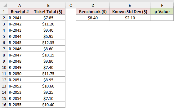
We want to test whether the average ticket total is higher than the benchmark.
Here is the formula:
=Z.TEST(B2:B16,D2,E2)
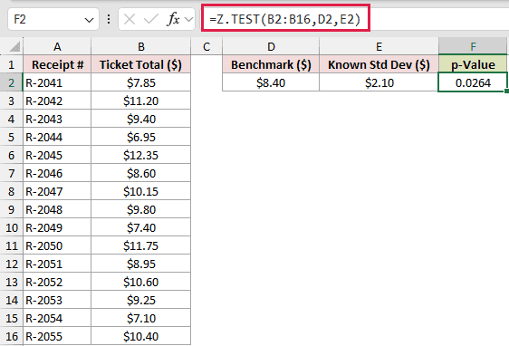
The formula returns 0.0264. That is below the chosen 0.05 significance level, so the sample supports an average ticket total above the $8.40 benchmark.
This conclusion answers an upper-tail question. You should choose that direction before inspecting the sample, not after seeing which test produces the smaller p-value.
Example 2: Omit Sigma When It Is Unknown
Z.TEST can also estimate variability from the sample.
Below is the dataset. Columns B:D contain drive-thru waits by daypart. The card in F:G holds the target wait and a labeled p-value cell.
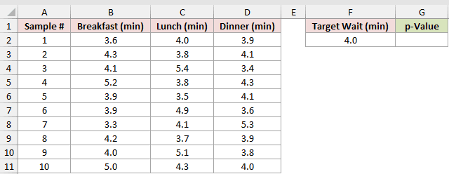
We want to test whether the average pooled wait is higher than the 4.0-minute target without supplying sigma.
Here is the formula:
=Z.TEST(B2:D11,F2)
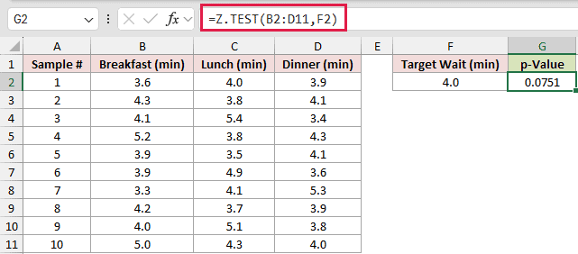
The formula pools all 30 wait times in B2:D11, covering 3 dayparts across 10 samples.
The returned p-value is 0.0751. It is above 0.05, so this sample does not provide enough evidence that the average pooled wait exceeds the target.
With this sample size, its sample standard deviation is a reasonable stand-in for sigma. For a small sample with an unknown population standard deviation, a t-test is generally better.
Example 3: Calculate a Two-Tailed p-Value
This example checks for movement in either direction.
Below is the dataset. Column B contains oven temperature readings. The D:G card has the set point, known standard deviation, and two labeled result cells.
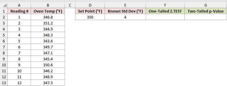
We first want Excel’s regular upper-tail result, then a valid two-tailed p-value.
Here is the one-tailed formula:
=Z.TEST(B2:B13,D2,E2)
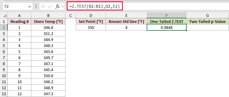
The upper-tail result is 0.9848 because the readings tend to fall below the set point.
Here is the two-tailed formula:
=2*MIN(Z.TEST(B2:B13,D2,E2),1-Z.TEST(B2:B13,D2,E2))
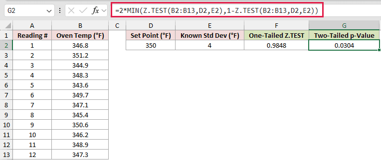
The MIN step chooses the smaller tail before doubling it. The resulting two-tailed p-value is 0.0304, which is below 0.05.
That result supports the conclusion that the average oven temperature differs from the set point, without assuming the direction beforehand.
Pro Tip: Do not double Z.TEST blindly. In this example, that produces 1.9696, which cannot be a probability. The MIN pattern checks the smaller tail first.
Example 4: Test Whether the Mean Is Lower
Now let’s ask a lower-tail question directly.
Below is the dataset. Columns A and B hold earbud units and battery-life readings. The D:F card contains the claim, known standard deviation, and lower-tail result cell.
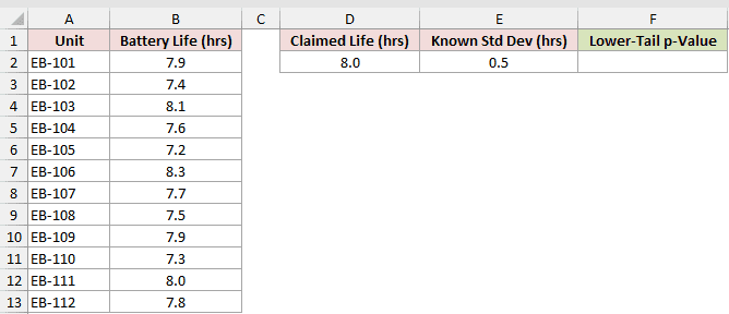
We want to test whether average battery life falls below the claimed level.
Here is the formula:
=1-Z.TEST(B2:B13,D2,E2)
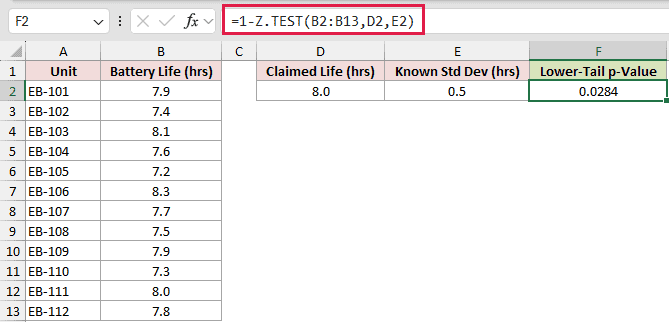
Z.TEST returns the upper tail, so subtracting it from 1 returns the lower tail. The result is 0.0284, which is below 0.05.
The same data produces a two-tailed p-value of 0.0567. Because this is above 0.05, the two-tailed test would not reject the null hypothesis.
Example 5: Report p, z, and the Decision
A useful test summary often needs more than the p-value.
Below is the dataset. Columns A and B hold orders and prep times. The D:F card contains the test inputs plus labeled cells for p, z, and the decision.
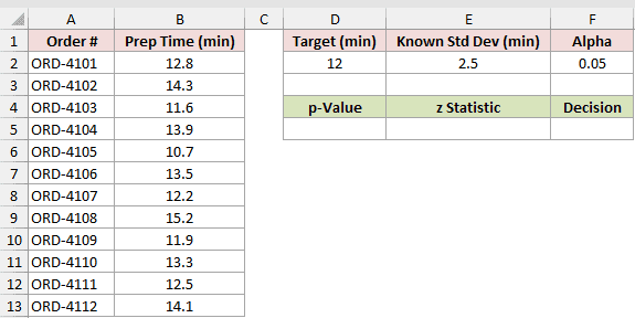
We want to calculate the p-value, recover the z statistic, and compare the result with alpha.
Here is the Z.TEST formula:
=Z.TEST(B2:B13,D2,E2)
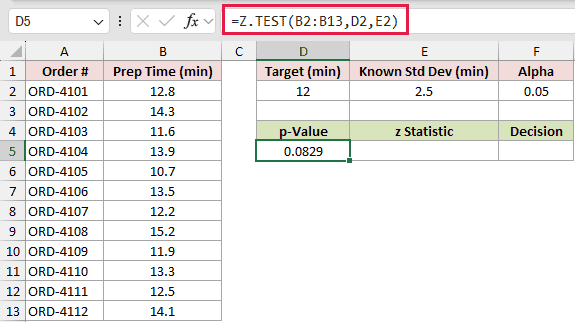
The p-value in D5 is 0.0829. Z.TEST returns only this probability, not the z statistic used to calculate it.
Here is the z-statistic formula:
=(AVERAGE(B2:B13)-D2)/(E2/SQRT(COUNT(B2:B13)))
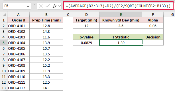
The formula standardizes the difference between the sample average and target. It returns a z statistic of 1.39.
Finally, here is the decision formula:
=IF(D5<F2,"Reject H0","Fail to reject H0")
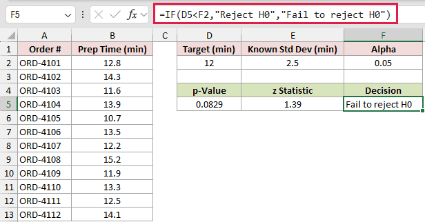
The formula compares 0.0829 with the 0.05 alpha in F2. It returns “Fail to reject H0” because the p-value is higher.
That wording matters. A result above alpha does not prove the target is correct. It means this sample does not provide enough evidence to reject it.
Example 6: Test One Group With FILTER
Here’s a practical way to test one group inside a longer list.
Below is the dataset. Columns A:C hold machine-cycle records. The E:H card identifies the machine, standard, known standard deviation, and labeled p-value cell.
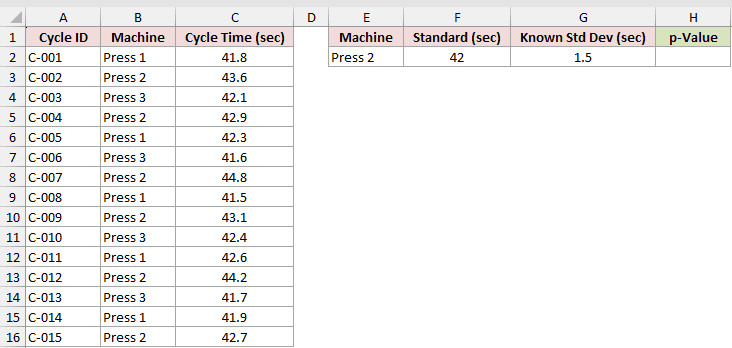
We want to test Press 2 without copying its records into a separate range.
FILTER requires Excel 2021, Excel 2024 or Microsoft 365.
Here is the formula:
=Z.TEST(FILTER(C2:C16,B2:B16=E2),F2,G2)
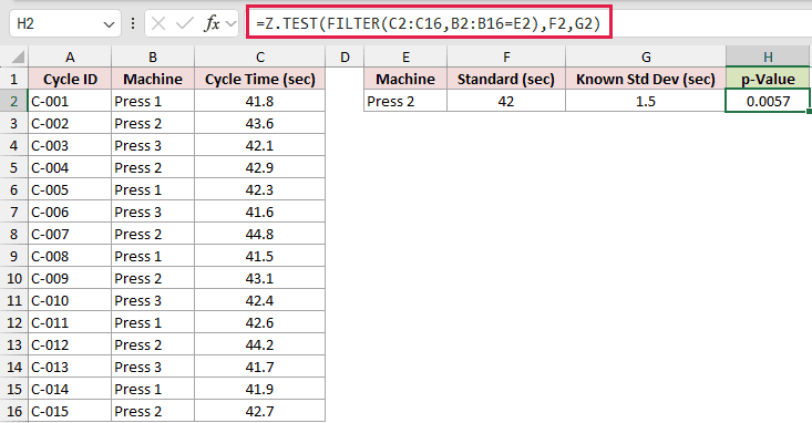
FILTER keeps the Press 2 cycle times, then Z.TEST reduces that filtered array to one p-value. The result is 0.0057.
Testing all cycles together returns 0.0566, which is above 0.05 and masks Press 2’s result.
Example 7: Test Several Benchmarks at Once
The final example changes the benchmark instead of the sample.
Below is the dataset. Columns A and B hold session records, D2:D6 contains benchmark inputs, G2 holds sigma, and E2:E6 is the result area.
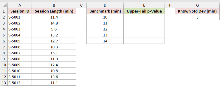
We want one formula to return an upper-tail p-value beside every benchmark.
This spilled result requires Excel 2021, Excel 2024 or Microsoft 365.
Here is the formula:
=Z.TEST(B2:B13,D2:D6,G2)
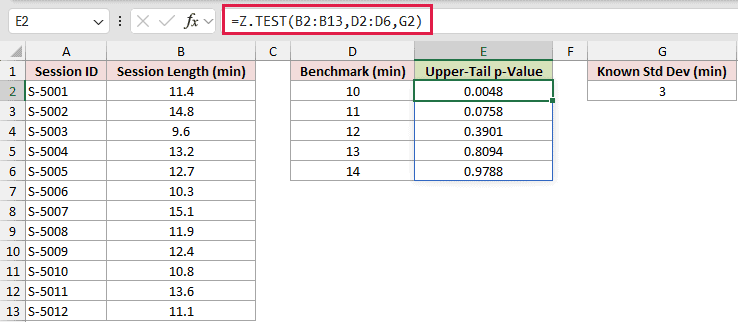
The formula spills 0.0048, 0.0758, 0.3901, 0.8094, and 0.9788 into E2:E6. Each result tests the same sample against its corresponding benchmark.
The sample mean is 12.24 minutes. The p-value passes 0.5 once the benchmark is higher than that mean.
Although Z.TEST normally reduces an array to one result, a range supplied for x can produce a spilled set of p-values.
Tips & Common Mistakes
- Z.TEST always returns the upper-tail p-value. Use the lower-tail or two-tailed patterns shown above when your question points elsewhere.
- Choose a one-tailed or two-tailed test before looking at the results. Changing direction afterward makes the evidence look stronger than it is.
- In testing, an empty array returned #N/A, one value with sigma omitted returned #DIV/0!, and sigma of 0 returned #NUM!.
- Text inside the sample range is ignored. Check imported data carefully because a text-formatted number could disappear from the test without an error.
- Z.TEST is a one-sample function. Comparing two groups requires a different method, such as the Analysis ToolPak’s two-sample z-test or an appropriate t-test.
- Z.TEST is available from Excel 2010. Excel 2007 and earlier use ZTEST. Use Z.TEST in new workbooks.
- If the spill area in Example 7 is blocked, Excel returns #SPILL!. Clearing E2:E6 lets the results appear without re-entering the formula.
I covered upper-tail tests with known sigma, along with what changes when you omit sigma or need a lower-tail or two-tailed result.
I also showed you how to report p, z, and the decision, test a filtered group, and spill p-values across several benchmarks.
Related Excel Functions / Articles:
