
Excel’s F.TEST function returns a two-tailed p-value for comparing the variances of two data samples.
It helps you judge whether their spreads differ significantly. It does not return the F statistic or identify which sample is more consistent.
In this article, I’ll show you how to interpret an F.TEST p-value, calculate the F statistic manually, and compare filtered groups.
F.TEST Function Syntax in Excel
The F.TEST function accepts two arrays or ranges containing the samples you want to compare.
=F.TEST(array1,array2)
- array1 (required) is an array or range of data holding the first sample.
- array2 (required) is an array or range of data holding the second sample.
When to Use F.TEST Function
- Check whether two machines produce measurements with different variability.
- Compare the consistency of two processes, routes, suppliers, or methods.
- Decide whether an equal-variance or unequal-variance T.TEST is more appropriate under a chosen rule.
- Compare groups stored in one table by passing filtered arrays to F.TEST.
Example 1: Compare Variance Between Two Machines
Let’s start with two machines filling bags to the same target weight.
Below is the dataset. Column A numbers the samples. Columns B and C hold the Machine A and Machine B fill weights (g).
The card shows the Calculation header and p-Value (F.TEST) label, plus the green Result header and empty result cell F2.
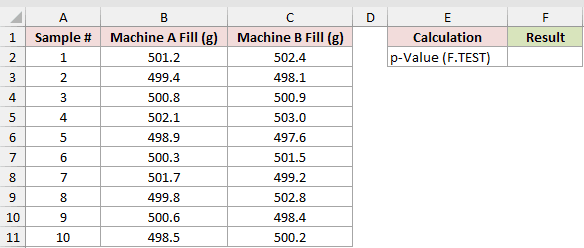
We want the two-tailed p-value for comparing the machines’ variances.
Here is the formula:
=F.TEST(B2:B11,C2:C11)
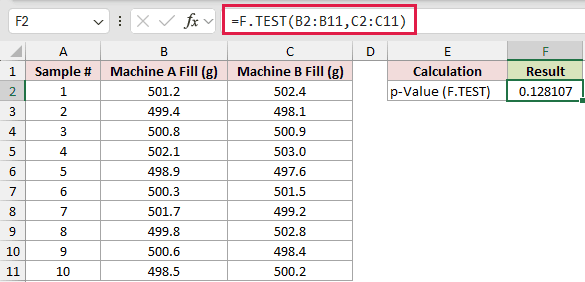
The formula returns 0.128107. Because that exceeds 0.05, these samples do not provide enough evidence that the machines have different variances.
Machine B’s readings look more spread out, but with ten bags per machine, the 0.128107 p-value is not low enough to call the difference significant.
Example 2: Interpret F.TEST Results at 0.05
Here’s a commute example where the two samples have different sizes.
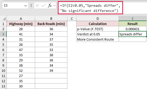
Below is the dataset. Columns A and B contain 12 highway times and 9 back-road times. The calculation card has three labels, a green Result header, and empty result cells.
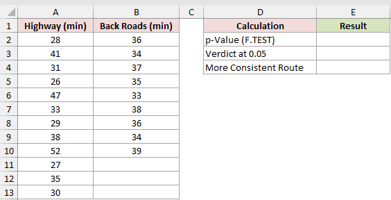
We want to test the spreads, return a verdict at 0.05, and identify the more consistent route.
First, calculate the p-value:
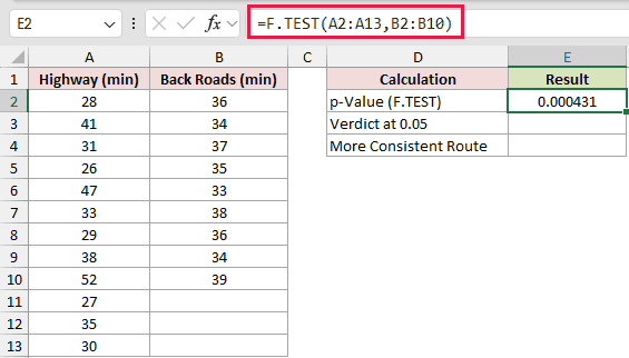
=F.TEST(A2:A13,B2:B10)
Next, turn the p-value into a plain-language verdict:
=IF(E2<0.05,"Spreads differ","No significant difference")
Finally, compare the sample standard deviations to find the more consistent route:
=IF(STDEV.S(A2:A13)<STDEV.S(B2:B10),"Highway","Back Roads")
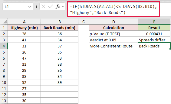
F.TEST returns 0.000431, so the verdict is Spreads differ. The unequal sample sizes do not prevent the calculation.
The final formula returns Back Roads. Its sample standard deviation is 1.9861 minutes, compared with 8.2696 minutes for Highway.
F.TEST detects a difference in spread, while STDEV.S shows which sample has less variation.
Example 3: Calculate the F Statistic Manually
Let’s unpack the calculation using readings from two thermometers in an ice bath.
Below is the dataset. Column A numbers the readings. Columns B and C hold ten readings from Thermometer A and Thermometer B.
The calculation card lists six measures beneath a green Result header, with every result cell empty.
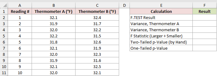
We want to compare F.TEST with a manual two-tailed calculation and a one-tailed result.
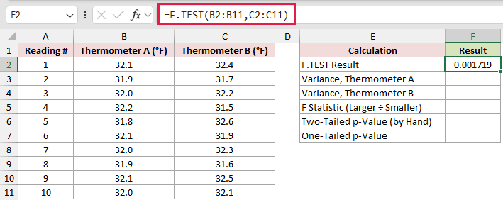
Start with the direct F.TEST result:
=F.TEST(B2:B11,C2:C11)
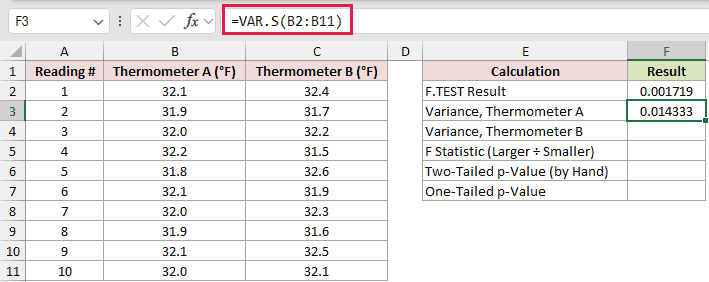
Now calculate the sample variance for Thermometer A:
=VAR.S(B2:B11)
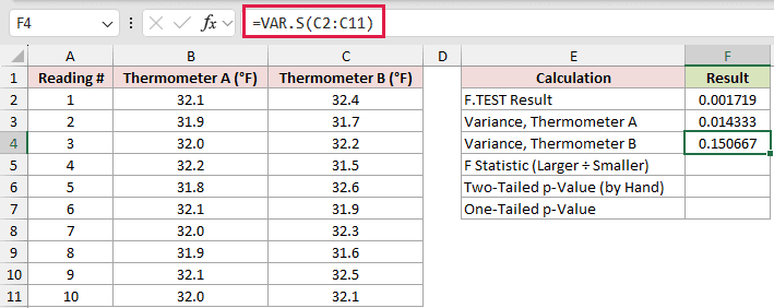
Then calculate the sample variance for Thermometer B:
=VAR.S(C2:C11)
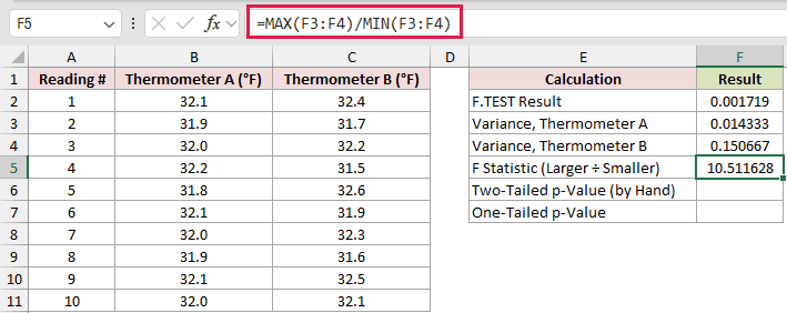
Divide the larger variance by the smaller one to get the F statistic:
=MAX(F3:F4)/MIN(F3:F4)
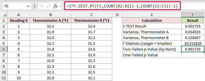
Use F.DIST.RT and double its result to reproduce the two-tailed p-value:
=2*F.DIST.RT(F5,COUNT(B2:B11)-1,COUNT(C2:C11)-1)
For comparison, remove the multiplication by 2 to return the one-tailed p-value:
=F.DIST.RT(F5,COUNT(B2:B11)-1,COUNT(C2:C11)-1)
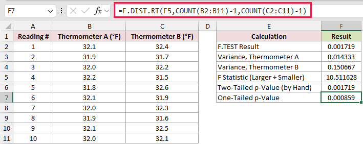
The sample variances are 0.014333 and 0.150667, producing an F statistic of 10.511628.
The manual two-tailed result is 0.001719, matching F.TEST. The one-tailed result is 0.000859, which is half the F.TEST result after rounding.
Both samples contain ten readings, so their degrees of freedom are equal.
F5 places Thermometer B’s larger variance in the numerator, but F6 and F7 use column B’s count as the first degrees-of-freedom argument.
That works here only because the counts match. With unequal counts, the first degrees-of-freedom argument must use the larger-variance sample’s count, which is column C here.
Pro Tip: The Data Analysis ToolPak’s F-Test reports a one-tailed probability. F.TEST returns a two-tailed p-value, so compare the correct result with your chosen significance level.
Example 4: Choose a T.TEST Type
Here’s one common workflow for comparing average runtimes from two suppliers.
Below is the dataset. Columns A and B contain 12 runtime values from each supplier. The calculation card has three labels, a green Result header, and empty result cells.
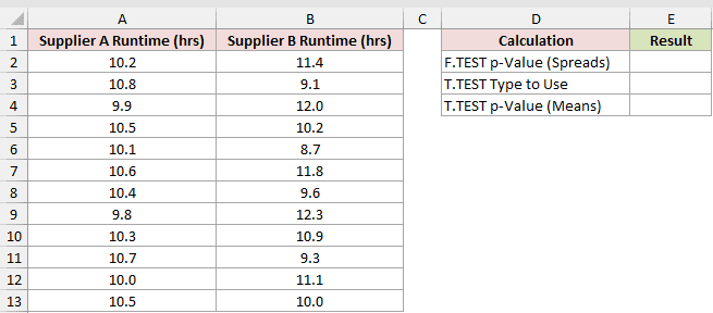
We want to test the variances, choose T.TEST type 2 or 3, and then compare the means.
First, calculate the F.TEST p-value:
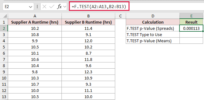
=F.TEST(A2:A13,B2:B13)
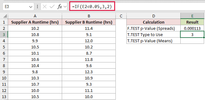
Next, return type 3 when the p-value is below 0.05, or type 2 otherwise:
=IF(E2<0.05,3,2)
Pass that result into the type argument of T.TEST:
=T.TEST(A2:A13,B2:B13,2,E3)
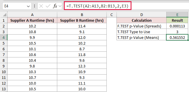
F.TEST returns 0.000113, so the IF formula returns 3. That tells T.TEST to use the unequal-variance method.
T.TEST then returns 0.561552. At 0.05, the samples do not show a significant difference between their mean runtimes.
Using F.TEST to choose the T.TEST type is one common convention. The choice remains optional because the F-test is sensitive to outliers and departures from normality.
Many analysts use the unequal-variance test by default, commonly called Welch’s t-test, instead of choosing a type from a preliminary F-test.
Example 5: Use F.TEST with FILTER
The final example compares two serving methods recorded in one table.
Below is the dataset. Columns A through C list 12 pours, their methods, and sizes.
The card shows the Calculation header and p-Value (Free Pour vs Jigger) label, plus the green Result header and empty result cell F2.
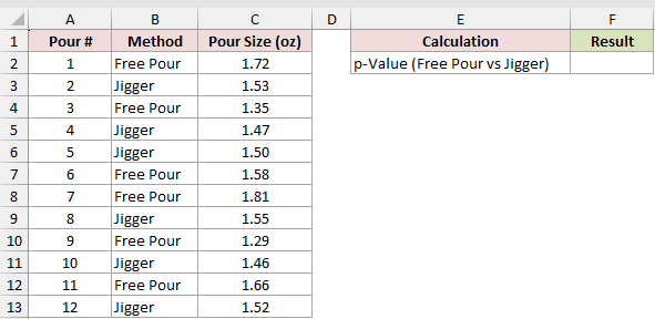
We want to compare the variance of Free Pour sizes with the variance of Jigger sizes.
Here is the formula:
=F.TEST(FILTER(C2:C13,B2:B13="Free Pour"),FILTER(C2:C13,B2:B13="Jigger"))
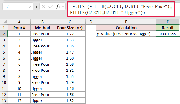
Each FILTER expression returns the pour sizes for one method. F.TEST compares those two arrays without helper columns.
The formula returns 0.001358. At 0.05, the sample variances are significantly different, although F.TEST alone does not identify which method varies more.
FILTER requires Excel 2021, Excel 2024, or Microsoft 365. F.TEST itself is available in Excel 2010 and later.
Tips & Common Mistakes
- F.TEST returns a two-tailed p-value, not the F statistic. Use VAR.S with F.DIST.RT when you need to see the underlying statistic.
- Compare the p-value with your chosen significance level. A result below 0.05 indicates significantly different variances when 0.05 is your cutoff.
- Swapping array1 and array2 does not change the F.TEST result.
- The sample ranges can have different lengths. Text inside a range is ignored.
- A sample with one numeric value or no variance returns
#DIV/0!. - F.TEST cannot tell you which sample is more consistent. Compare VAR.S or STDEV.S results for direction.
- Use F.TEST for new work. The older FTEST function remains available for compatibility and returns the same result.
- The F-test assumes roughly normal data and is sensitive to outliers, so review the data before relying on its p-value.
F.TEST gives you a compact way to judge whether two samples have different spreads.
Use STDEV.S or VAR.S to see which sample varies more.
Use F.DIST.RT for the F statistic route, or T.TEST to compare means.
Related Excel Functions / Articles:
