How to Lock a Row in Excel

If you want to lock a row in Excel, the first thing to work out is which kind of locking you actually mean. The phrase covers three completely different jobs, and Excel handles each one with a different feature.

That’s why searching for it turns up answers that have nothing to do with your problem. But nothing to worry about.

Once you know which of the three you’re after, each one takes seconds. In this article I’ll show you eight ways to lock a row in Excel, grouped by what you’re trying to do.

Lock a Row So It Stays Visible While Scrolling in Excel

This is what most people mean. You scroll down, your headers slide off the top of the screen, and you lose track of which column is which.

Freezing pins a row to the top of the window so it never scrolls away.

Method #1: Use Freeze Top Row to Lock a Row in Excel

This is the fastest option in Excel, and it needs no selection at all. One click and row 1 is pinned.

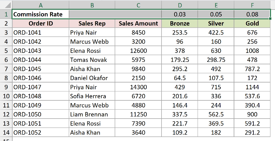
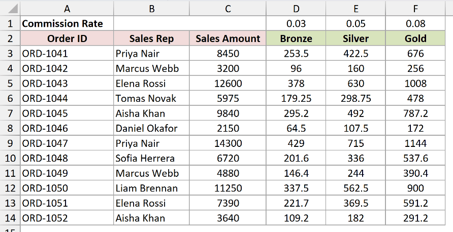
Below I have a commission sheet. Row 1 holds the three commission rates in D1, E1, and F1 (0.03, 0.05, and 0.08).

Row 2 has the column headers, and rows 3 to 14 have the orders. I want the rates to stay on screen while I scroll through the orders.

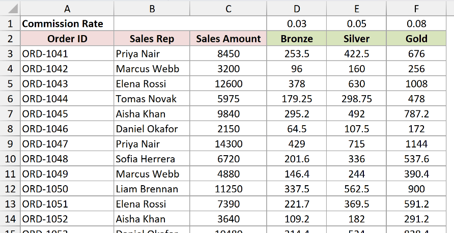
Here are the steps to lock the top row:

1. On the View tab, click Freeze Panes, then click Freeze Top Row.

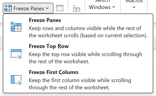
2. Scroll down through the orders. Row 1 stays pinned at the top.

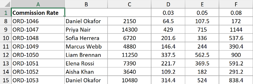
Watch row 2 as you scroll, though. Row 1 is pinned, but row 2 slid away with everything else.

Freeze Top Row only ever freezes row 1. My headers are in row 2, so this isn’t enough. Method #2 fixes that.

Note: On Windows you can do this from the keyboard with Alt + W + F + R. Those ribbon accelerators are Windows-only, since Excel for Mac has no Alt ribbon navigation. There’s more on the keyboard route in Freeze Pane in Excel (Shortcut).

Method #2: Use Freeze Panes to Lock Multiple Rows in Excel

This is the one I’d recommend, and it’s really the only rule you need to learn.

Freeze Panes freezes everything above the row you select, and everything to the left of the column you select. The selected row itself is not included.

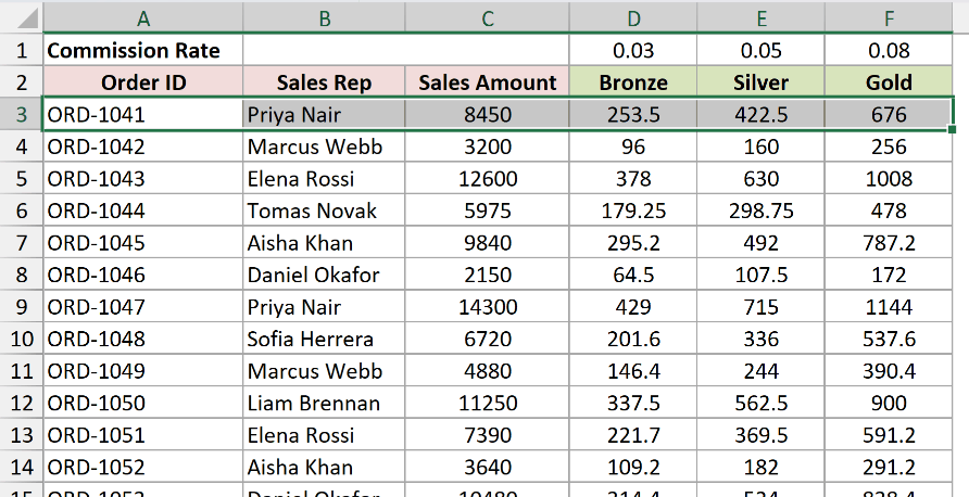
So to freeze rows 1 and 2, you select row 3.

Below I have the same commission sheet. Row 1 holds the rates, row 2 holds the column headers, and rows 3 to 14 hold the orders. This time I want both row 1 and row 2 to stay on screen.

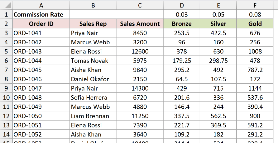
Here are the steps to lock multiple rows:

1. Click the row header for row 3 to select the whole row. Rows 1 and 2 sit above it, so those are the two that will freeze.

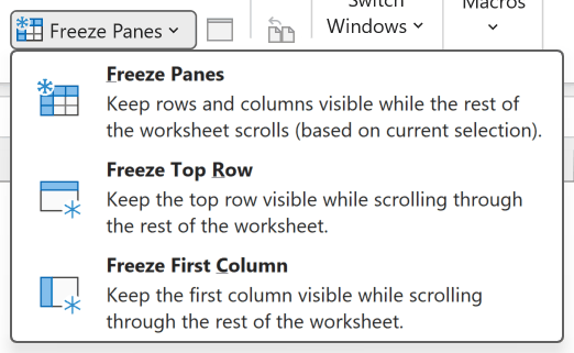
2. On the View tab, click Freeze Panes, then click Freeze Panes again in the drop-down.

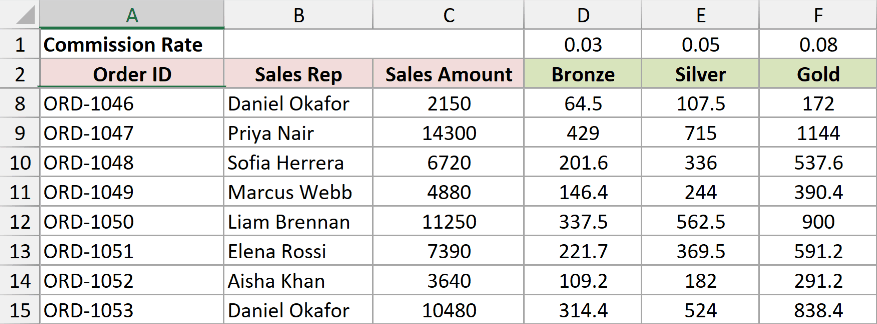
3. Scroll down. Rows 1 and 2 both stay put, with a thin grey line marking where the freeze sits.

Once that rule clicks, Method #1 stops looking like a separate feature. Freeze Top Row is just this method with row 2 selected for you.

That’s why I reach for Freeze Panes every time. It handles one row, five rows, or a row and a column together, all with the same click.

Note: If your data sits in an Excel Table (Ctrl + T), Excel swaps the column-letter strip for your header labels as you scroll. That is not the same as locking a row. It only works while the active cell is inside the Table, and it stops working the moment Freeze Panes is switched on.

Freezing the first column, freezing a row and a column together, and unfreezing again all follow from the same rule. I’ve walked through each of those in How to Freeze the Top Row and First Column in Excel.

If you’d rather automate it, there’s a code version in VBA to Freeze Top Row in Excel.

Method #3: Use the Split Feature to Lock a Row in View in Excel

Here’s another way to keep a row in sight, and it’s the one to use when you want to compare two parts of the same sheet.

Split cuts the window into panes that scroll independently. The top pane holds your row still while you move around in the bottom one.

Below I have the same commission sheet. The rates are in row 1, the headers are in row 2, and the orders run from row 3 to row 14. I want rows 1 and 2 held in a pane of their own.

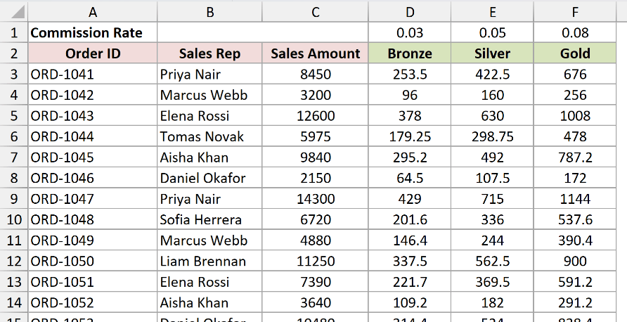
Here are the steps to split the window:

1. Click cell A3. The divider drops in right above whichever cell you have selected.

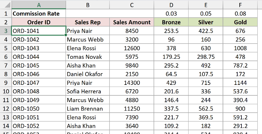
2. On the View tab, click Split.

3. Scroll inside the lower pane. Rows 1 and 2 sit still in the top pane while the orders move.

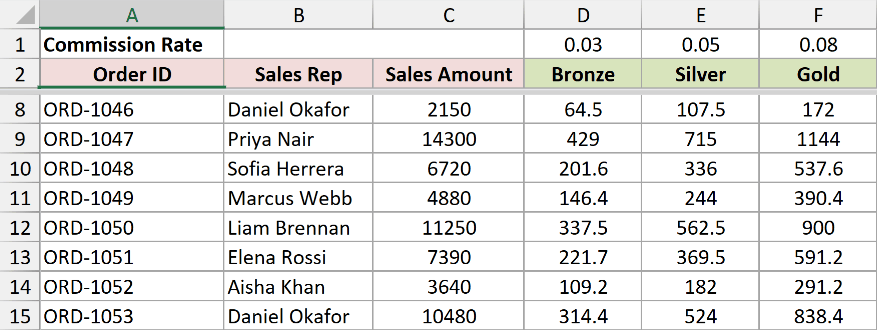
The difference from freezing is that a split pane still scrolls. You can move the top pane to row 40 if you want to line two sections up side by side.

To get rid of the divider, double-click it, or click Split again.

Note: Freeze Panes and Split can’t both be on at once. Turning one on clears the other automatically, so don’t go hunting for a bug when your freeze disappears after a split.

Lock a Row So It Cannot Be Edited in Excel

This one has nothing to do with the screen. You want the row to sit there and refuse to change, no matter who clicks on it.

Method #4: Lock the Row With Format Cells and Protect Sheet in Excel

This is the real answer to “stop people editing my row”, and the order of the steps is the whole thing.

The part that trips everyone up is what Excel starts you with. Every cell in a new sheet is already set to Locked. That setting just does nothing until you protect the sheet.

So if you jump straight to Protect Sheet, you don’t lock one row. You lock all of them.

The fix is to unlock everything first, then lock only the row you care about, and protect the sheet last.

Below I have the commission sheet. The rates live in row 1, and I want to stop anyone typing over them while rows 3 to 14 stay open for new orders.

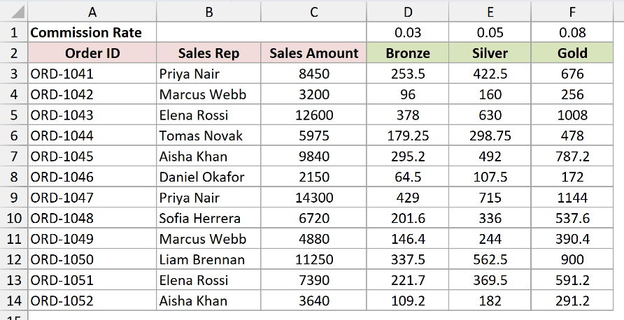
Here are the steps to lock a row against edits:

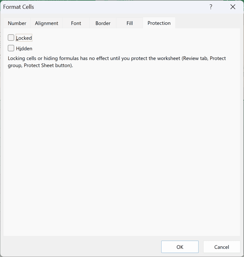
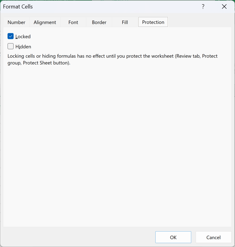
1. Press Ctrl + A to select every cell on the sheet, press Ctrl + 1 to open Format Cells, go to the Protection tab, and uncheck Locked. Click OK.

2. Click the row 1 header to select the whole row.

3. Press Ctrl + 1 again, go to the Protection tab, and this time check Locked. Click OK.

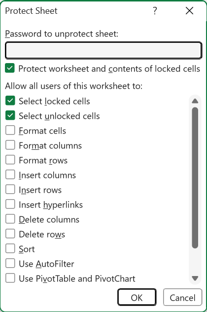
4. On the Review tab, click Protect Sheet. Add a password if you want one, and click OK.

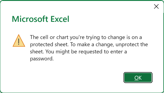
5. Try typing in D1. Excel blocks it with a warning, while rows 3 to 14 still take edits normally.

Skip step 1 and the sheet goes read-only from top to bottom. Skip step 4 and nothing is locked at all.

Note: The Locked checkbox has no effect on its own. Until you run Protect Sheet, every cell stays editable no matter how that box is set. This is why so many people tick Locked, test it, and conclude it’s broken.

What you just did to a row works the same on single cells, columns, and whole sheets. For the wider version, including the password options, see How to Lock Cells in Excel.

There’s also a keyboard route to the Locked setting in Lock Cells in Excel (Shortcut).

Method #5: Use Allow Edit Ranges to Lock a Row in Excel

This one reaches the same place from the opposite direction.

Instead of unlocking everything and re-locking one row, you leave every cell Locked, which is how they already are, and carve out the ranges people are allowed to edit. Row 1 stays locked because you never touched it.

You can also give each carved-out range its own password, which Method #4 can’t do.

Note: Allow Edit Ranges is Windows-only. The button has never been added to the Review tab in Excel for Mac, so use Method #4 if you’re on a Mac.

Below I have the commission sheet again. The rates are in row 1, and I want row 1 locked while everything from row 2 down stays editable.

Here are the steps to lock a row with Allow Edit Ranges:

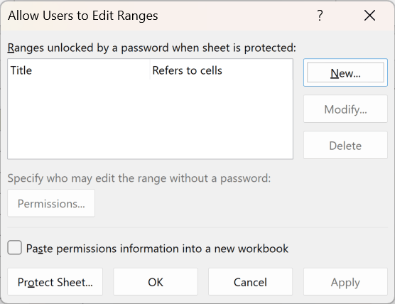
1. On the Review tab, click Allow Edit Ranges.

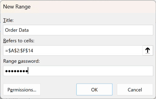
2. Click New. In the New Range dialog, type a title such as Order Data, set Refers to cells to =$A$2:$F$14, and type a range password. Click OK, then re-enter the password to confirm.

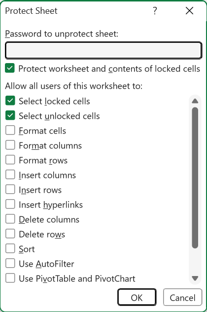
3. Back in the Allow Edit Ranges dialog, click Protect Sheet at the bottom, set a sheet password, and click OK.

4. Click any cell in the order rows and start typing. Excel asks for the range password and lets you through. Row 1 gives you no prompt at all.

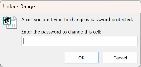
The range password is optional. Leave it blank and the range is simply editable with no prompt, which gets you the same result as Method #4 in fewer clicks.

Method #6: Use a VBA Macro to Lock a Row in Excel

If you set the same row lock up every week, or across a stack of sheets, the four dialogs in Method #4 get old fast. A macro does the lot in one keypress.

Below I have the commission sheet. The rates are in row 1, and I want the macro to lock that row and protect the sheet, leaving the rest editable.

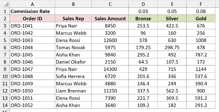
Here is the VBA code:

Sub LockRowOne()
    Dim ws As Worksheet
    Set ws = ActiveSheet

    ws.Unprotect
    ws.Cells.Locked = False
    ws.Rows(1).Locked = True
    ws.Protect
End Sub

Sub LockRowOne()
    Dim ws As Worksheet
    Set ws = ActiveSheet

    ws.Unprotect
    ws.Cells.Locked = False
    ws.Rows(1).Locked = True
    ws.Protect
End Sub

Here are the steps to use this macro:

1. Press Alt + F11 to open the VBA Editor
2. Insert a new module (Insert → Module)
3. Paste the code above
4. Press F5 to run the macro

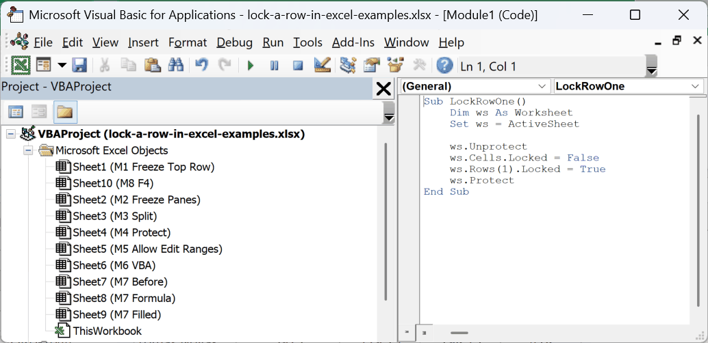
The code walks through Method #4 in the same order, which is why it works. ws.Unprotect clears any existing protection so the Locked settings can be changed. ws.Cells.Locked = False unlocks every cell.

ws.Rows(1).Locked = True then locks row 1 on its own, and ws.Protect switches the protection on so the setting takes effect.

Change Rows(1) to whichever row you need, or to something like Rows("1:2") for two rows. For a password, use ws.Protect Password:="yourpassword" on the last line.

Note: Save the workbook as a macro-enabled file (.xlsm) if you want to keep the macro. Save it as a regular .xlsx and Excel throws the code away.

Lock a Row Reference in an Excel Formula

The third meaning has nothing to do with the screen or with protection. It’s about stopping a row number from shifting when you copy a formula somewhere else.

Method #7: Add a Dollar Sign to Lock a Row Reference in Excel

Copy a formula down a column and Excel helpfully moves every reference down with it. That’s usually what you want. When the formula points at a rate sitting in row 1, it isn’t.

A dollar sign in front of the row number pins that row in place.

Below I have the commission sheet. The three rates are in D1, E1, and F1, the sales amounts are in column C, and I want to work out each order’s commission at all three rates in D3:F14.

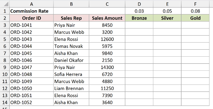
Here is the formula for cell D3:

=$C3*D$1

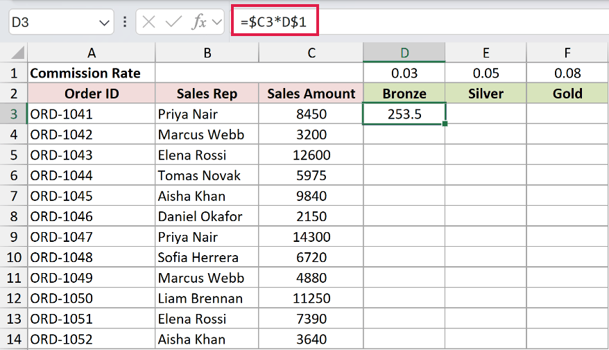
Now copy D3 and paste it across and down into D3:F14. Every cell fills with the right commission.

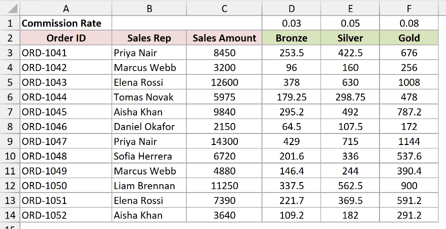
How does this formula work?

Look at D$1 first. The dollar sign sits before the row number, so the row is pinned to 1 and the column letter is free to move.

Copy the formula across to E3 and it becomes E$1. Still row 1, but now the Silver rate. Copy it to F3 and it’s F$1, the Gold rate. The reference walks Bronze to Silver to Gold and never leaves row 1.

Now $C3 does the mirror image. The dollar sign is before the column letter, so the column is pinned to C and the row is free.

Copy down to D4 and it becomes $C4, the next order’s sales amount. It walks down the orders and never leaves column C.

Put them together and D3 gives 8450 × 0.03 = 253.50. E3 gives 8450 × 0.05 = 422.50, and F3 gives 8450 × 0.08 = 676.

Drop the dollar sign from D$1 and copying to row 4 would point at D2, which is empty. Every commission in the table would come out as 0.

A reference that pins only the row or only the column is called a mixed reference. There’s a fuller breakdown of what the symbol does in What does $ (dollar sign) mean in Excel Formulas?.

Pin both halves at once and you get an absolute reference, which is covered in What is Absolute Cell Reference in Excel?.

Method #8: Use the F4 Shortcut to Lock a Row Reference in Excel

Typing dollar signs by hand gets old somewhere around the third formula. F4 puts them in for you.

Below I have the same commission sheet, with the rates in row 1 and the sales amounts in column C. This time I’ll build the row lock with the keyboard instead of typing it.

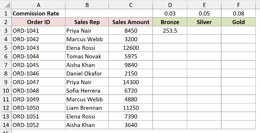
Here are the steps to lock a row reference with F4:

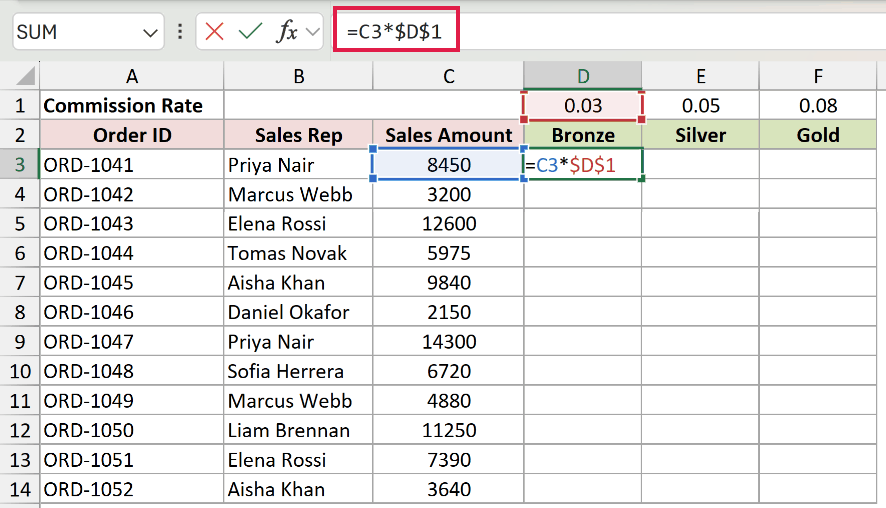
1. Double-click cell D3 to put it in edit mode, and click inside the D1 part of the formula so the cursor is sitting on that reference.

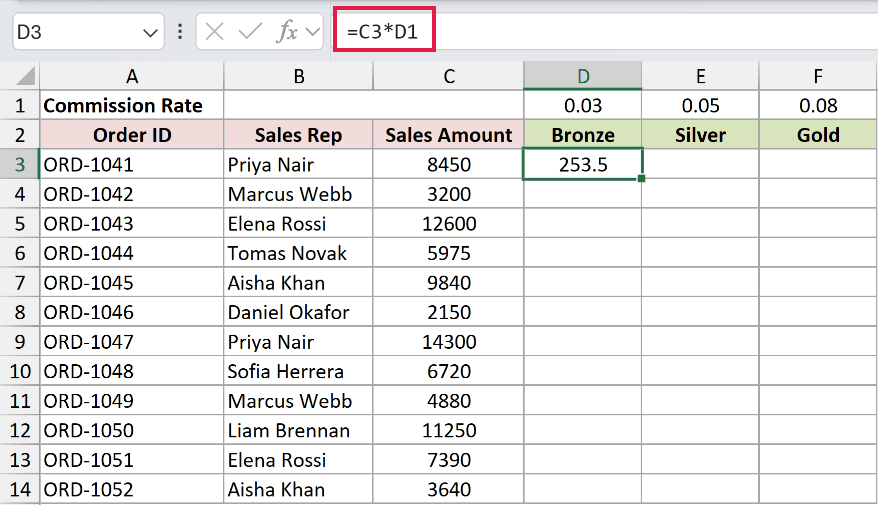
2. Press F4 once. D1 becomes $D$1, with both the column and the row pinned. That’s one too many dollar signs.

3. Press F4 again. It becomes D$1, which is the row lock you want. Press Enter.

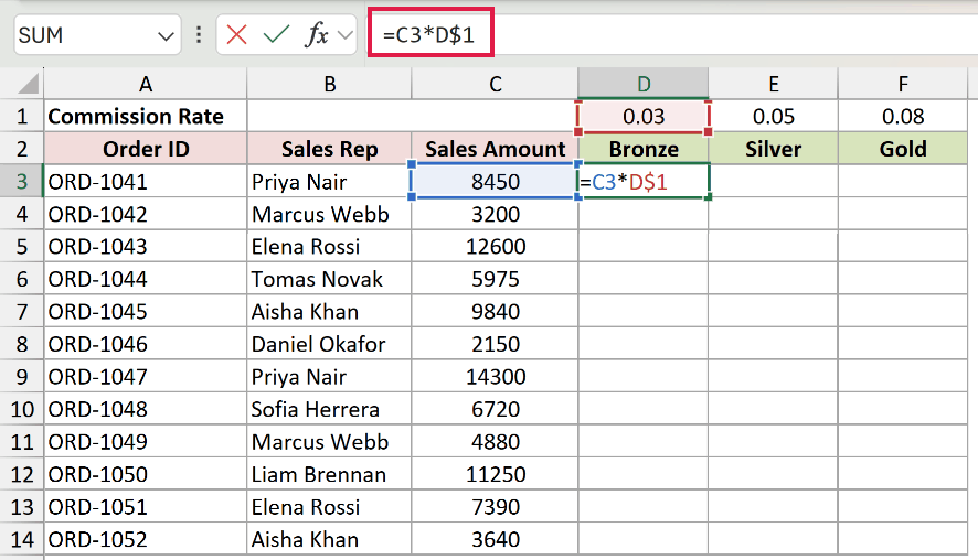
The full cycle runs D1 to $D$1 to D$1 to $D1, and then back to D1.

That order is worth memorising, because it means the row lock is always the second press. Land on $D1 and you’ve gone one too far, so keep pressing until it comes round again.

The $C3 half of the formula is the same trick, three presses in. Park the cursor on C3 and press F4 three times.

Note: On a Mac, F4 does nothing while you’re editing a formula. The cycle is Command + T there instead. Fn + F4 works only if you’ve set the function keys to behave as standard function keys.

The same key cycles the column lock and the fully-pinned version too, and I’ve laid out all four states in Toggle Between Cell References (Absolute/Relative/Mixed) Shortcut.

Additional Notes About Locking a Row in Excel

• Freeze Panes and Split are set per worksheet, not per workbook. Freezing row 1 on one sheet leaves every other sheet in the file untouched, so you have to repeat it on each one.
• Freeze and Split can’t both be on at once. Turning one on clears the other, so you can’t have a frozen row and a split pane together.
• Protect Sheet prevents accidents, not attacks. It is not encryption. It stops a colleague overwriting your rates by mistake, so don’t lean on it to hide anything sensitive.
• Freezing a row does nothing to your printout. A frozen row still prints once, on page one. Repeating a header on every printed page is a separate setting, covered in How to Set a Row to Print on Every Page in Excel.

Frequently Asked Questions

Does freezing a row stop people from editing it?

No. Freeze Panes only changes what stays on screen. The row is still a normal row, and anyone can click it and type straight over it. Stopping edits is a separate feature, and that’s Method #4.

Why is the Freeze Panes option greyed out in Excel?

Usually because the sheet is in Page Layout or Page Break Preview view. Switch to Normal on the View tab and the option comes back. It’s also greyed out while a cell is in edit mode, so press Esc first if you were mid-formula.

Why doesn’t F4 work when I try to lock a row reference?

Two common reasons. On a Mac, F4 doesn’t cycle references at all, so use Command + T. On Windows, the cell has to be in edit mode with the cursor on the reference. Outside edit mode, F4 repeats your last action instead.

How do I unlock a row after protecting the sheet?

On the Review tab, click Unprotect Sheet and type the password if you set one. Everything is editable again straight away. Your Locked settings stay as they were, so protecting the sheet again brings the same row lock back.

Conclusion

Locking a row in Excel means three different things, and picking the right one takes seconds once you know which is which.

If you want the row to stay on screen, use Freeze Panes and select the row below the last one you want pinned. If you want to stop people editing it, unlock everything, lock the row, then protect the sheet, in that order.

And if you’re writing a formula, D$1 is the one you’re after.

Other Excel articles you may also like:

• How To Go to the Top of the Page in Excel (Shortcuts)
• Row vs Column in Excel – What’s the Difference?
• How to Turn OFF Scroll Lock In Excel?
• Arrow Keys Not Working in Excel (Not Moving Between Cells)