When you bring in data from other sources, it is not uncommon to get the dates in the form of serial numbers, like 42088.
Moreover, Excel inherently stores dates in the form of integers and then formats it according to the required date settings.
So when you apply certain formulas to dates or when you format a cell in the Number format, you often end up getting a serial number.
Although this form of storing dates seems unintuitive, it makes sense because it’s easier for Excel to perform various calculations with dates when in integer form.
Since it’s difficult for us humans to understand this date format though, it becomes necessary to convert these serial numbers to a recognizable date format.
In this tutorial, we will see three ways to convert a serial number to date format in Excel.
Understanding the Concept of Serial Numbers
Excel stores date in the form of integers or serial numbers. The serial starts from January 1, 1900, and increases by 1 for each day since then. That means January 1, 1900, has the serial 1, the next day has the serial 2, and so on.
In this way, the serial for June 1, 2019, is 43617, because it is exactly 43,617 days after January 1, 1900.
How to Convert Serial Numbers to Date in Excel
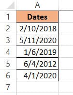
Throughout this tutorial, we are going to use the following set of date serial numbers.
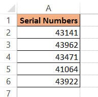
We will use the above three methods to convert these serial numbers to dates in different formats.
Method 1: Converting Serial Number to Date using the TEXT function
The TEXT function in Excel converts any numeric value (like date, time, and currency) into text with the given format. We can use this function to convert our serial number to any date format.
Here’s the syntax for the TEXT function:
= TEXT (serial_number, date_format_code)
In this function,
- serial_number is the numeric value or reference to the cell that you want to convert.
- date_format_code is the date format you want to convert the serial number to.
The TEXT function essentially applies the date_format_code that you specified on the provided serial_number and returns a text string with that format. For example, if you have the serial number “43141” in cell A2, then =TEXT(A2,”dd/mm/yy”) will return “10/02/18”
The format code will depend on the format that you want your converted date to appear. Here are some basic building blocks for the format codes that you can use:
Format Codes for Day of the Month:
You can use the following basic format codes to represent day values:
- d – one or two-digit representation of the day (eg: 3 or 30)
- dd – two-digit representation of the day (eg: 03 or 30)
- ddd – the day of the week in abbreviated form (eg: Sun, Mon)
- dddd – full name of the day of the week (eg: Sunday, Monday)
So,
- if you apply =TEXT(A2, “d”) to the sample dataset, it will return “10”.
- if you apply =TEXT(A2, “dd”), then it will return “10”.
- if you apply =TEXT(A2, “ddd”) to the sample dataset, it will return “Sat”.
- if you apply =TEXT(A2, “dddd”), then it will return “Saturday”.
Format Codes for Year:
You can use the following basic format codes to represent year values:
- yy – two-digit representation of year (e.g. 20 or 12)
- yyyy – four-digit representation of year (e.g. 2020 or 2012)
So,
- if you apply =TEXT(A2, “yy”) to the sample dataset, it will return “18”.
- if you apply =TEXT(A2, “yyyy”), then it will return “2018”.
Format Codes for Month of the Year:
You can use the following basic format codes to represent month values:
- m – one or two-digit representation of the month (eg; 8 or 12)
- mm – two-digit representation of the month (eg; 08 or 12)
- mmm – month abbreviated in three letters (eg: Aug or Dec)
- mmmm – month expressed with the full name (eg: August or December)
So,
- if you apply =TEXT(A2, “m”) to the sample dataset, it will return “2”.
- if you apply =TEXT(A2, “mm”), then it will return “02”.
- if you apply =TEXT(A2, “mmm”), then it will return “Feb”.
- if you apply =TEXT(A2, “mmmm”), then it will return “February”.
Let us see how we can apply the TEXT function to our sample dataset to convert all the serial numbers to different date formats.
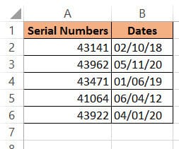
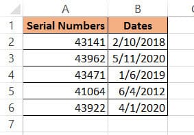
We will first see how to convert the serial numbers in column A to the format shown in column B in the image below:
Below are the steps to do this:
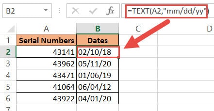
- Click on a blank cell where you want the converted date to be displayed (B2)
- Type the formula:
=TEXT(A2,”mm/dd/yy”).
- Press the Return key.
- This should display the serial number in our required date format. Copy this to the rest of the cells in the column by dragging down the fill handle or double-clicking on it.
- Copy this column’s formula results by pressing CTRL+C or Cmd+C (if you’re on a Mac).
- Right-click on the column and form the popup menu that appears, press Paste Values from the Paste Options.
- This will store the formula results as permanent values in the same column. Now you can go ahead and remove column A if you want to.
The result you get in column B will differ according to the format code you used in step 2. Here are some format codes along with the type of result you will get when applied to cell A2:
| Function | Result |
| =TEXT(A2, “dd/mm/yy”) | 02/10/18 |
| =TEXT(A2, “mm-dd-yy”) | 02-10-18 |
| TEXT(A2,”dddd, mmmm d, yyyy”)”) | Saturday, February 10, 2018 |
This means you can use the TEXT function to convert serial numbers to any date format of your choice. All you need to do is change the format_code according to your requirement.
Note: Using this formula, your converted date is in text format. If you want to convert it to date format, you need to use the Format Cells feature.
Also read: How To Combine Date and Time in Excel (3 Easy Ways)
Method 2: Converting Serial Number to Date using Format Cells
This method makes use of Excel’s FormatCells dialog box. The Format Cells dialog box is very versatile and lets you perform different kinds of formatting from one place.
You can use Format Cells to convert the serial numbers in our sample dataset into dates as follows:
- Select all the cells containing the serial numbers that you want to convert (A2:A6).
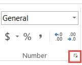
- Right-click on your selection and select Format Cells from the popup menu that appears. Alternatively, you can select the dialog box launcher in the Number group under the Home tab.
- This will open the Format Cells dialog box. Click on the Number tab
- Under Category on the left side of the box, select the Date option.
- This will display a number of formatting options for the date on the right side.
- Select the format that you want.
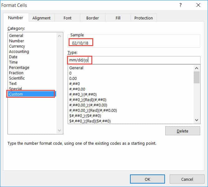
- If you don’t find an option for the format you want to use, then you can use the Custom option from the Category list on the left. This lets you convert the cell to a custom date format.
- Check if your required date format is available among the format codes under Type. If not, you can type in your format code in the input box just below Type.
- Click OK to close the Format Cells dialog box.
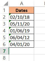
All your selected cells should now be converted to date with your required format.
Note that these cells do not have the little green triangles at the top left corners. This is because these cells are of type date, and not text. So, you can perform any kind of date operations on them.
Also read: How to Add Minutes to Time in Excel?
Method 3: Converting Serial Number to date using VBA
If you’re comfortable with coding or using VBA, then you can use this method to quickly get all your serial numbers converted to date in one go.
Here’s the VBA code. You can copy and save this code somewhere for future use:
Sub convert_serial_num_to_date()
Dim rng As Range
Dim cell As Range
Set rng = Application.Selection
For Each cell In rng
cell.Offset(0, 1).Value = CDate(cell.Value)
Next cell
End Sub
Here are the steps you need to follow if you want to apply the above code to your dataset:
- From the Developer Menu Ribbon, select Visual Basic.
- Once your VBA window opens, Click Insert->Module. Now you can start coding. Type or copy-paste the above lines of code into the module window. Your code is now ready to run.
- Go to your worksheet and select the range of cells containing the serial numbers you want to convert. Make sure the column next to it is blank because this is where the code will display the results.
- Navigate to Developer->Macros-> convert_serial_num_to_date->Run.
You will now see the serial numbers converted to dates in the column next to your selection.
If you want to, you can now delete the original column containing the serial numbers.
In this tutorial, we saw three simple ways in which you can convert date serial numbers to actual dates in Excel. These included the use of the TEXT function, the Format Cells feature, and the VBA script.
Using the TEXT function usually results in cells that are of the text format so it requires subsequent conversion of these cells to the date format.
Using Format Cells, however, you can apply the operation directly on the original cells and the results you get are of the date type. So, you can directly start applying the cells to date-related operations. T
The VBA script that we provided in this tutorial used CDate() to quickly convert the serial number to its date equivalent. Moreover, the script results in cells that are of type date.
So again, it’s easier to use these results in subsequent date operations.
We hope you found the pointers we provided in this tutorial helpful and easy to apply.
Other Excel tutorials you may like:
- How to Convert Date to Month and Year in Excel
- How to Convert Decimal to Fraction in Excel
- How to Add Consecutive Numbers in Excel
- How to Convert Radians to Degrees in Excel
- How to Add Days to a Date in Excel
- How to Sort by Date in Excel (Single Column & Multiple Columns)
- How to Convert Date to Day of Week in Excel
- How to Convert Month Number to Month Name in Excel
- Find Last Monday of the Month Date in Excel
- How to Change Date and Time to Date in Excel