Want to supercharge your Excel lookups?
Wildcards in XLOOKUP let you match fragments of text, hunt down partial entries, and return accurate results even when you don’t know the full lookup value.
It’s one of the simplest ways to make your searches smarter, faster, and more flexible.
I will show you how to use wildcards in XLOOKUP.
Using Wildcards in XLOOKUP
The syntax of XLOOKUP is:
XLOOKUP(lookup_value, lookup_array, return_array, [if_not_found], [match_mode], [search_mode])
To enable wildcard support in XLOOKUP, set the [match_mode] argument to 2.
The table below shows you when to use each wildcard.
| Use | To find |
|---|---|
| * (asterisk) | Any sequence of characters, including zero characters. For instance, *west finds ‘Northwest’ and ‘Southwest.’ |
| ? (question mark) | Any single character. For instance, A?e finds ‘Axe’ and ‘Ace.’ |
| ~ (tilde) followed by *, ?, or ~ | An asterisk, a question mark, or a tilde. For example, zp90~* finds ‘zp90*’ |
Example #1: Use the Asterisk (*) Wildcard in XLOOKUP
Suppose you have the price list below.
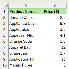
You want to find out the price of the first item on the list whose name begins with ‘App’.
Use the formula below to return the price you are looking for.
=XLOOKUP(D3,A2:A10,B2:B10,"Not found",2)
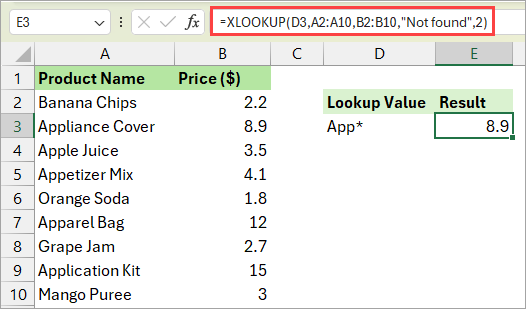
The lookup value in cell D3 is ‘App*’, with the asterisk placed at the end.
The formula returns 8.9, the price of the first matching item, ‘Appliance Cover’.
Note: You can place the asterisk wildcard at the beginning, end, or both sides of the lookup value. For example, to return the price of the first item whose name ends with ‘over’, use the lookup value ‘*over’ (asterisk at the beginning).
To find the first item whose name contains ‘ran’, you would use ‘*ran*’ (asterisks on both sides).
Also read: How to Replace Asterisks in Excel
Example #2: Use the Question Mark (?) Wildcard in XLOOKUP
Let’s say you have the product status report below.
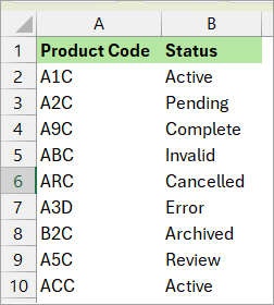
You want to find out the status of the first product on the report whose three-letter product code begins with B and ends with C.
Use the formula below to return the status of the target product.
=XLOOKUP(D3,A2:A10,B2:B10,"Not found",2)
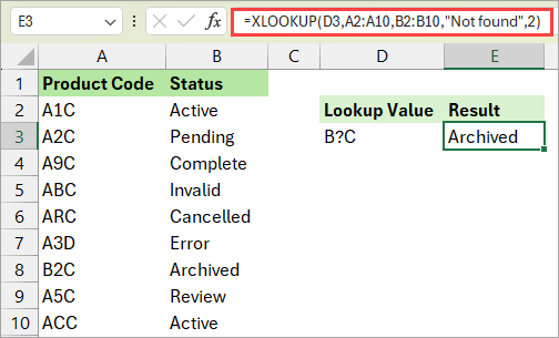
The look_up value in cell D3 is ‘B?C’.
The formula returns ‘Archived’, the status of the first product on the list whose three-letter code is B2C.
Example #3: Use the Tilde (~) Wildcard in XLOOKUP
Suppose you have the report below.

Use the formula below to return the owner of the first ‘Plan*2025’ in the dataset.
=XLOOKUP(D3,A2:A10,B2:B10,"Not found",2)
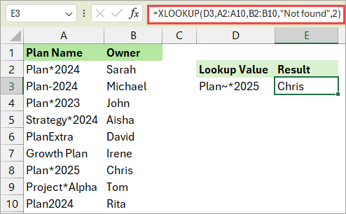
The look_up value in cell D3 is ‘Plan~*2025’.
The formula returns ‘Chris’, the owner of the ‘Plan*2025’ in the dataset.
I have shown you how to use wildcards in XLOOKUP. I hope you found the tutorial helpful.
Other Excel articles you may also like: