
The IFS function in Excel checks conditions in order and returns the value associated with the first TRUE condition.
It can replace nested IF formulas for ordered rules, such as score bands. Put more restrictive conditions first when several could be true.
In this article, I’ll show you how to assign grades, calculate tiered commissions, and choose shipping costs from weight bands.
IFS Function Syntax in Excel
Here is what the IFS function looks like.
=IFS(logical_test1, value_if_true1, [logical_test2, value_if_true2], ...)
- logical_test1, value_if_true1 (required): The first condition to test and the value to return if that condition is TRUE.
- [logical_test2, value_if_true2] (optional): More condition/value pairs, added as needed.
- IFS returns the value of the first test that comes back TRUE and then stops.
- You can add up to 127 condition/value pairs in a single formula.
One thing to keep in mind: IFS has no built-in “else” argument. To catch everything that didn’t match a condition, use TRUE as the final logical_test and give it a default value.
When to Use IFS Function
IFS is handy any time you need to sort a value into one of several buckets. A few common cases:
- Turning scores into letter grades (A, B, C, D, F).
- Setting a tiered commission or discount rate based on a sales or order amount.
- Creating status labels from a number, like stock levels or progress.
- Pricing shipping by weight band.
- Assigning performance ratings from a KPI or review score.
Example 1: Assign Letter Grades
Let’s start with the classic grading example.
Below is the dataset with student names in column A, their scores in column B, and an empty Grade column in C.
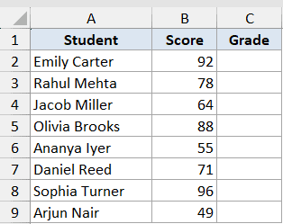
We want to convert each score into an A through F letter grade.
Here is the formula:
=IFS(B2>=90,"A",B2>=80,"B",B2>=70,"C",B2>=60,"D",TRUE,"F")
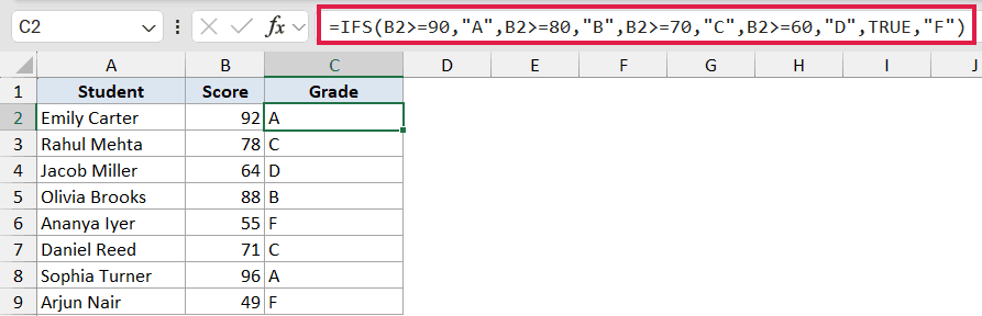
How this formula works:
- IFS tests the conditions from highest to lowest, in order.
- If B2 is 90 or more, it returns “A” and stops. If not, it checks 80, then 70, then 60.
- The final pair,
TRUE,"F", acts as the catch-all. Any score under 60 lands here and gets an “F”.
Enter the formula in C2, then fill it down the column to grade everyone.
Pro Tip: Always add TRUE as the last condition. Without it, any row that matches none of your tests returns a #N/A error instead of a clean default value.
Example 2: Grade the Class in One Formula
If you’re on Excel 365, you can rate everyone at once instead of filling a formula down.
Below is the dataset with employee names in column A, their KPI scores in column B, and an empty Rating column in C.
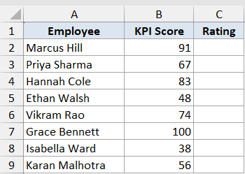
We want a single formula that rates the whole team and spills the results down.
Here is the formula:
=IFS(B2:B9>=85,"Excellent",B2:B9>=70,"Good",B2:B9>=50,"Average",TRUE,"Needs Improvement")
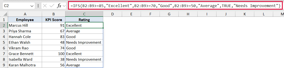
How this formula works:
- Instead of pointing at one cell, each test points at the full range B2:B9.
- Excel 365 reads the whole column and applies the same logic to every row.
- You type the formula once in C2, and the results spill automatically down C2:C9. No fill-down needed.
This is the dynamic-array version of the same grading idea, and it keeps your sheet to a single formula.
Example 3: Tiered Sales Commission
IFS works just as well with numbers as the return value.
Below is the dataset with rep names in column A, their sales in column B, and an empty Commission Rate column in C.
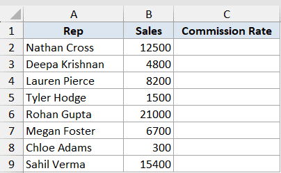
We want to assign a commission rate based on which sales band each rep falls into.
Here is the formula:
=IFS(B2>=20000,0.15,B2>=10000,0.1,B2>=5000,0.07,B2>=1000,0.03,TRUE,0)
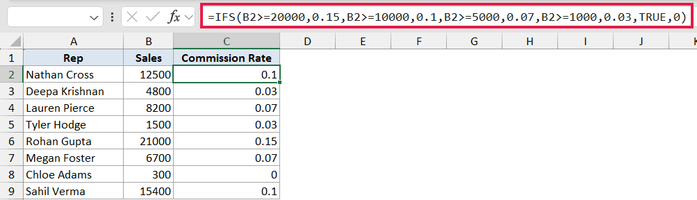
How this formula works:
- The bands run from highest to lowest. IFS checks 20000 first, then 10000, then 5000, then 1000.
- The high-to-low order matters. If you listed the lowest band first, every rep would match it and the higher tiers would never be reached.
- The
TRUE,0pair gives anyone below 1000 a rate of 0.
If you want the result to read as a percentage, format the Commission Rate column as a percentage.
Example 4: Stock Status From Quantity
You can use IFS to turn a plain number into a readable label.
Below is the dataset with product names in column A, the quantity on hand in column B, and an empty Status column in C.
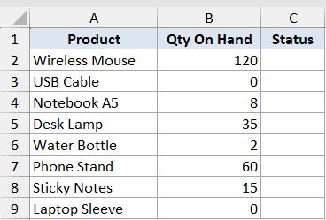
We want to convert each quantity into a stock status label.
Here is the formula:
=IFS(B2>=50,"In Stock",B2>=10,"Low Stock",B2>=1,"Critical",TRUE,"Out of Stock")
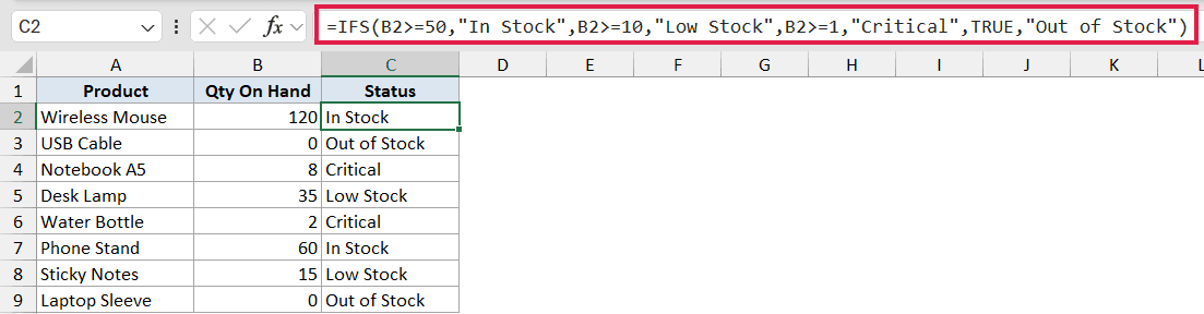
How this formula works:
- 50 or more reads as “In Stock”, 10 to 49 as “Low Stock”, and 1 to 9 as “Critical”.
- The
TRUE,"Out of Stock"pair catches anything that didn’t match, which means a quantity of 0 (or even a negative number) gets labeled “Out of Stock”.
This shows why the catch-all is worth setting. A value of 0 fails every numeric test above, so without the TRUE pair it would return an error instead of a useful label.
Example 5: Shipping Cost by Weight
Sometimes your tiers go the other direction, from low to high.
Below is the dataset with order IDs in column A, each order’s weight in column B, and an empty Shipping Cost column in C.
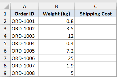
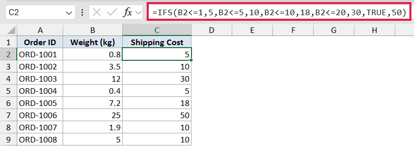
We want to price each order by its weight band.
Here is the formula:
=IFS(B2<=1,5,B2<=5,10,B2<=10,18,B2<=20,30,TRUE,50)
How this formula works:
- This one uses
<=and lists the bands in ascending order, from light to heavy. - It’s the mirror image of the grade and commission examples, which used
>=from high to low. - The catch-all
TRUE,50prices anything over 20 kg at 50.
Getting the direction right is what makes the tiers work. With <= you go low to high. With >= you go high to low. Mix them up and the first matching test will grab everything.
Pro Tip: Order matters because IFS stops at the first TRUE result. Whether you sort high-to-low with >= or low-to-high with <=, line your tests up so the most specific band is reached before the broader ones.
Example 6: IFS vs SWITCH for Exact Matches
IFS can also map exact values, though it’s not always the tidiest tool for that job.
Below is the dataset with shift lead names in column A, a day number from 1 to 7 in column B, and an empty Day Name column in C.
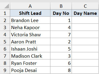
We want to convert each day number into a short day name.
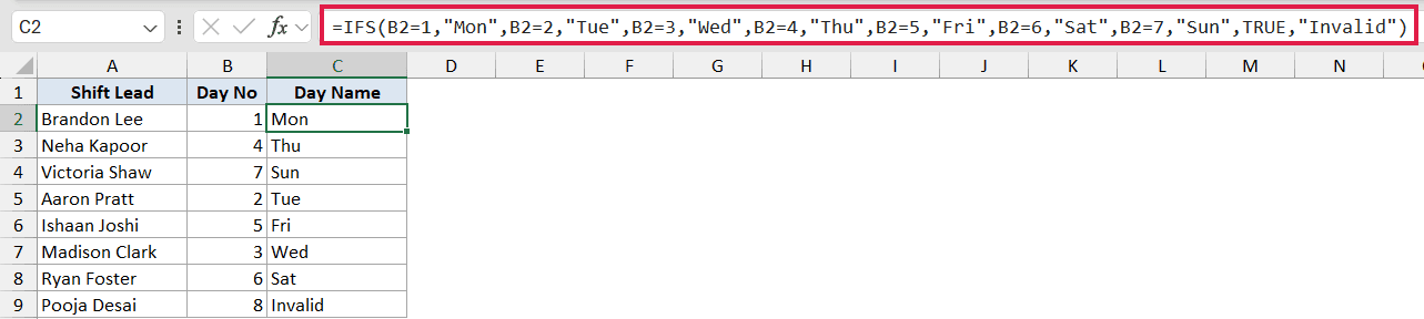
Here is the formula:
=IFS(B2=1,"Mon",B2=2,"Tue",B2=3,"Wed",B2=4,"Thu",B2=5,"Fri",B2=6,"Sat",B2=7,"Sun",TRUE,"Invalid")
How this formula works:
- Each test compares B2 against one exact number and returns the matching name.
- The row with Day No 8 matches none of the numbers, so it hits
TRUE,"Invalid".
When you’re testing one value against a list of exact options like this, SWITCH is usually cleaner. You name the cell once and it has a built-in default, so you skip repeating B2= over and over:
=SWITCH(B2,1,"Mon",2,"Tue",3,"Wed",4,"Thu",5,"Fri",6,"Sat",7,"Sun","Invalid")
A simple rule of thumb: use IFS when your conditions are ranges (>, <, >=), and use SWITCH when you’re mapping one value to discrete exact results.
Tips & Common Mistakes
- Always add
TRUE, valueas the final pair. Without it, rows that match no condition return a #N/A error. - Order matters. IFS returns the first TRUE result, so arrange your threshold tests from most to least restrictive.
- IFS needs Excel 2019, 2021, or 365. Older versions return a #NAME? error.
- IFS has no else argument the way IF does, so the TRUE catch-all is how you set a default.
- For mapping one value to discrete exact results, SWITCH is usually tidier than IFS.
IFS turns a tangle of nested IFs into something you can read top to bottom. Test your conditions in the right order, add a TRUE catch-all, and you’ll get clean results every time. When you’re matching exact values instead of ranges, reach for SWITCH instead.
Related Excel Functions / Articles:
- Excel Logical Test Using Multiple If Statements in Excel [AND/OR]
- Using IF Function with Dates in Excel (Easy Examples)
- CHOOSE Function in Excel
- COUNTIFS Function in Excel
- SUMIFS Function in Excel
- IFERROR Function in Excel
- How to use Excel If Statement with Multiple Conditions Range [AND/OR]
- How to Use Greater Than or Equal to Operator in Excel Formula?
