
If you have a column of percentages in Excel, getting a single average feels like it should be a quick AVERAGE and done. The catch is that a plain average can mislead you when each one came from a different sample size.
The good news is Excel handles both the quick version and the accurate version. You just need to know which one your data needs.
In this guide I’ll show you four ways to calculate an average percentage, including the weighted formula that stays honest when the row totals differ.
Method #1: Using the AVERAGE Function
The AVERAGE function is the one most people try first, and for good reason. You point it at your column of percentages and it hands back the mean.
It’s the right call when every row is measured against the same base, and a fine gut-check even when it isn’t.
If you want a fuller tour of the function itself, take a look at our guide to the AVERAGE function in Excel.
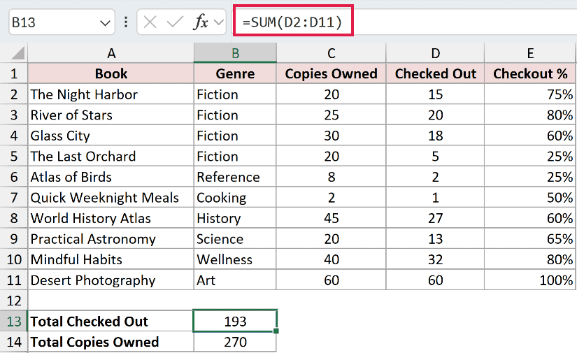
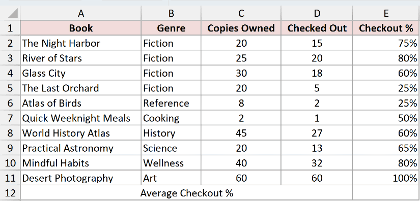
Below is my library catalog. Each row is a book, and columns C and D hold the total copies owned and how many are currently checked out.
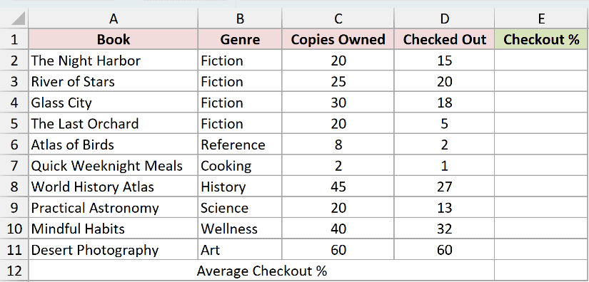
First I add a Checkout % column in E with =D2:D11/C2:C11. The formula spills down the column automatically, and I format the range as a percentage so each title shows its own checkout rate.
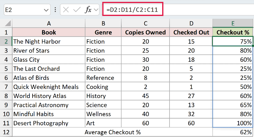
Now for the average. Here is the formula:
=AVERAGE(E2:E11)
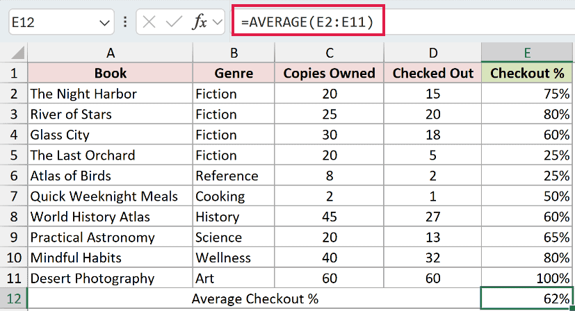
How does this formula work?
AVERAGE adds up the ten percentages in E2:E11 and divides by 10. That gives 62%, the plain mean of the checkout rates. Every book counts equally here, whether it has 8 copies on the shelf or 60.
Note: A plain AVERAGE treats every row as equal weight. If your percentages come from different totals, jump to Method #2 for the number that reflects the real counts.
Method #2: Using a Weighted Average Formula
Here’s the method I reach for when the per-row totals aren’t the same. A weighted average goes back to the raw numbers instead of averaging the percentages.
You add up all the copies checked out, add up all the copies owned, and divide one total by the other. That way a book with 60 copies pulls more weight than one with 8, which is exactly what you want.
Using the same library catalog, I want one checkout percentage that reflects the whole collection, not just the average of the per-title rates.
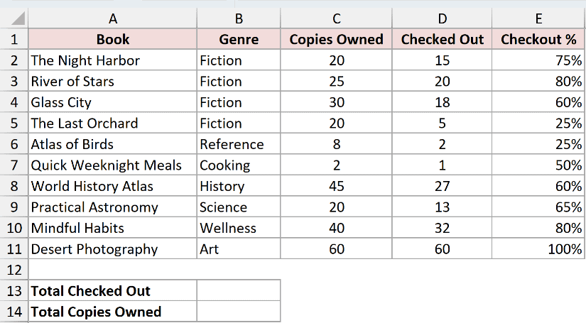
It helps to see the two totals on their own first. =SUM(D2:D11) gives 193 copies checked out, and =SUM(C2:C11) gives 270 copies owned.
Here is the formula that combines them:
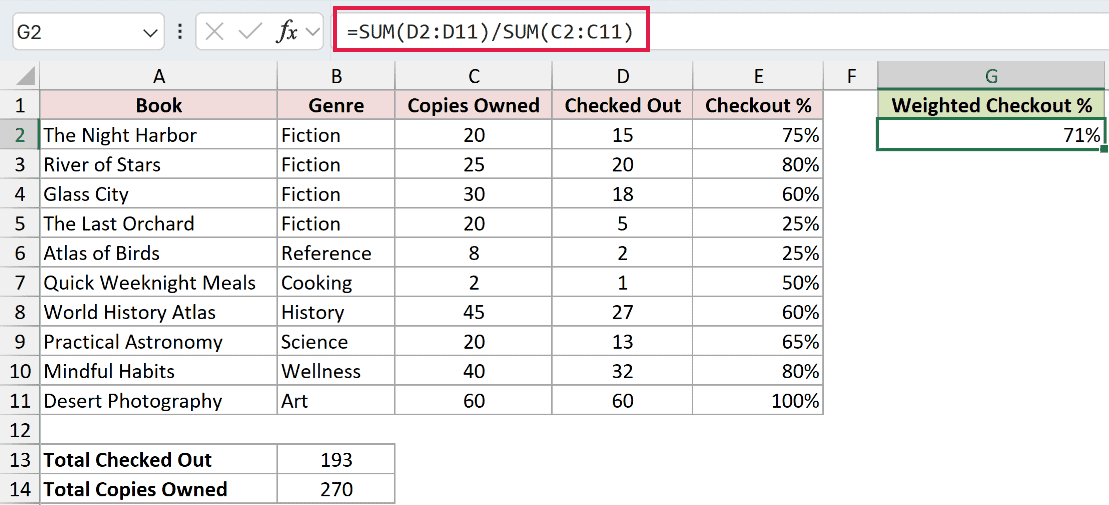
=SUM(D2:D11)/SUM(C2:C11)
How does this formula work?
SUM(D2:D11) totals the copies checked out, 193. SUM(C2:C11) totals every copy owned, 270. Dividing gives 0.7148, or about 71% once the cell is formatted as a percentage.
Notice it lands nine points above the plain average from Method #1. That’s the busy, high-copy titles finally carrying their real weight.
Note: The division returns a decimal like 0.7148. Format the result cell as Percentage (Home tab, then the % button) so Excel shows it as 71% instead of a raw number.
Method #3: Using AVERAGEIF Function
Sometimes you don’t want the whole table averaged, just one slice of it. AVERAGEIF averages only the rows that match a condition you set.
Same library catalog, and this time the Genre column in B does the filtering. I want the average checkout percentage for the Fiction books on their own.
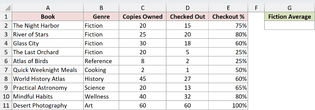
Here is the formula:
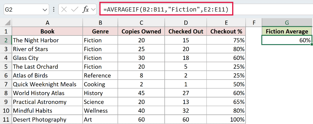
=AVERAGEIF(B2:B11,"Fiction",E2:E11)
How does this formula work?
AVERAGEIF looks down B2:B11 for the word Fiction, and for every match it pulls the matching percentage from E2:E11. Four books are tagged Fiction, with rates of 75%, 80%, 60%, and 25%. Their average works out to 60%.
Note: The same weighting caveat applies inside a category. If the Fiction titles have very different total copies, use =SUMIF(B2:B11,”Fiction”,D2:D11)/SUMIF(B2:B11,”Fiction”,C2:C11) for the weighted rate instead of AVERAGEIF.
Method #4: Using the AutoSum Drop-Down
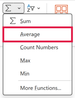
If you’d rather not type a formula at all, Excel can write the AVERAGE for you. The AutoSum drop-down on the Home tab has an Average option built in.
You select a cell, pick Average, and Excel drops the formula in and guesses the range above it. It’s the fastest way to a quick average percentage.
Back to the full library catalog. I want the average of the checkout percentages in column E, using the ribbon instead of typing anything.
Here are the steps to calculate the average percentage with AutoSum:
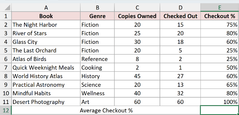
- Select the cell right below your percentages, which is E12 in this catalog.
- On the Home tab, in the Editing group, click the drop-down arrow next to AutoSum and choose Average.
- Check that Excel picked up the range E2:E11, then press Enter.
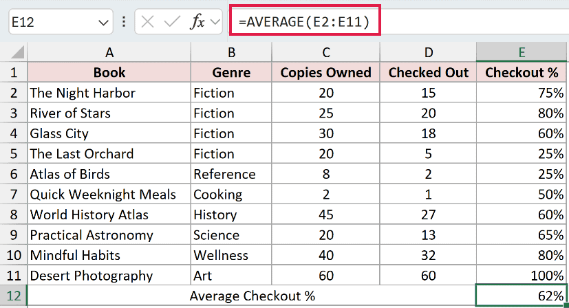
Excel writes =AVERAGE(E2:E11) for you and returns 62%, the same plain mean you got in Method #1.
Additional Notes About Calculating Average Percentage in Excel
- Percentages stored as text won’t average. If a cell shows 75% but sits left-aligned, Excel is treating it as text and AVERAGE will skip it. Re-enter it as a number or run it through VALUE first.
- AVERAGE ignores blank cells but counts zeros. An empty percentage is left out of the math, while a genuine 0% row pulls the mean down, so know which one you actually have.
- Watch the display versus the true value. A cell can read 71% while the real number is 71.48%. Add decimal places or wrap the result in ROUND before you report it anywhere.
- Plain AVERAGE ignores filters. If you’ve filtered the list, use
=SUBTOTAL(1,E2:E11)so only the visible rows are averaged.
Frequently Asked Questions
Why does a simple average of percentages give a misleading result?
Say one title has 5 copies and another has 500. A plain average gives both the same say, so the 5-copy book can swing your number far more than its size deserves. That distortion is why uneven bases need a weighted calculation.
How do I average percentages that come from different sample sizes?
When rows have different totals, don’t average the percentage column directly. If you have each row’s percentage and a weight, =SUMPRODUCT(E2:E11,C2:C11)/SUM(C2:C11) multiplies each rate by its weight and divides by the total, giving the weighted result without the raw counts.
Can I format the AVERAGE result as a percentage automatically?
If the cells you’re averaging are already formatted as percentages, the result usually inherits that format. If it shows a decimal like 0.62 instead, select the cell and press Ctrl+Shift+%, or click the % button on the Home tab.
Conclusion
Averaging percentages in Excel comes down to one question: do all your rows share the same base? If they do, a plain =AVERAGE or the AutoSum drop-down gets you there in seconds.
If they don’t, reach for the weighted formula in Method #2, since it’s the only one that reflects the real totals. And when you just need one category, AVERAGEIF keeps things tidy.
Other Excel articles you may also like:
