Imagine you bring home your test scores and you’re really happy with how you’ve scored…up until one of your parents asks you ‘what percentile is it?’ or ‘what’s the cumulative percentage of your score’?
That’s probably when you realize that you haven’t really scored as well as you thought!
Jokes aside, the cumulative percentage gives you one way to express or analyze a frequency distribution.
Using this, you can get a good idea of the percentage of values in the distribution that lie above or below a given value.
In this tutorial we will show you 3 ways to compute the cumulative percentage for different values (or intervals) in a given distribution:
- By Manual Computation
- Using a Formula
- Using a Pivot Table
What is Cumulative Percentage and What is it Used For?
Simply put, the cumulative percentage of a value or interval is the percentage of the cumulative frequency for that value (or interval) in a given distribution.
It can also be considered as a sort of running total of a percentage value, where the percentage increases with each value.
The last value in the distribution (highest value) always has a cumulative percentage of 100%.
As such, it gives us a good idea of how the percentages in a frequency table add up over a time period.
For example, let’s say a dice was rolled 30 times and the following is the frequency distribution obtained:

If we know the cumulative percentage for each number in this distribution, we can tell how many times the dice rolled a number (say) between 1 and 4.
This can help us understand how probable it is to roll a number below 4.
So say after computing the cumulative percentage, this is the result we got:

From the above result, we can tell that around 70% of the time the dice rolled a number below 4.
This can help us easily that there is a high probability of rolling a number below 4.
Similarly, you can use the cumulative percentage to find out what percentage of students scored below a given score.
If you find that the cumulative frequency of, say, 75 is 30%, it means that 30% of the students who gave the test scored below 75. You could also say that 70% of the students scored more than 75.
Of course, the applications of the cumulative percentage are not just limited to these two.
It is a widely used statistical analysis tool used in a number of industries, including scientific research finance, banking, and more.
Also read: How to Add a Percentage to a Number in Excel?
How to Calculate the Cumulative Percentage for a Frequency Distribution
As mentioned before, the cumulative percentage is basically a running total of percentage values.
So for each value, you have to find the frequency percentage of one period and add to it the frequency percentage of the previous periods.
Let’s see how the calculation is done manually. Let’s say you have the frequency distribution of student test scores as follows:

To find the cumulative percentage, you first need to compute the cumulative frequency of each score.
The cumulative frequency of each value is simply the total frequency of values including and below the said value, as shown below:

You can then compute the cumulative percentage of a value by dividing the cumulative frequency of the value by the total frequency, then multiplying by 100.
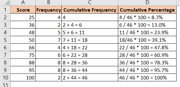
So the cumulative percentage of , say, 50 is 18 / 46 * 100 = 39.1%.
Also read: How to Calculate Growth Rate in Excel
How to Calculate Cumulative Percentage in Excel
Of course, instead of manually computing the cumulative percentage, you can automate the process using Excel. There are 3 ways to get this done:
- By Manual Computation
- Using a Formula
- Using a Pivot Table
Let us see each of these methods one by one. We will demonstrate each method using the same frequency distribution table:

Using Manual Computation to Calculate Cumulative Percentage in Excel
The first method uses simple manual computation to find the cumulative percentage.
We mentioned this method first, as it can help you clearly see how cumulative percentage computations are basically done.
Before finding the cumulative percentage in this method, we need to first compute the cumulative frequencies for each value.
So you will need to insert a helper column that will calculate the cumulative frequencies first.
Here are the steps:
- Create a helper column for Cumulative frequency.

- Type the formula: =SUM($B$2:B2) in the first cell (C2) of this column. We locked the cell reference B2 into an absolute reference because when the formula is copied down to the other cells of the column, each time, we want to sum up values starting from cell B2 up to the current row.

- Copy this formula down to the rest of the cells using the fill handle.

- You should now see column C populated with cumulative frequencies corresponding to each test score. The last value in this column (46) is the total frequency (in this case, the total number of students that were tested).
- Create a new column to compute the cumulative percentage.

- Type the formula: =C2/$C$10 in cell D2. Here, we are dividing the cumulative frequency of the test score 25 by the total frequency. We locked the cell reference C10 with dollar symbols because we want this reference to remain the same when the formula is copied down to the rest of the cells in the column.

- Copy this formula down to the rest of the cells using the fill handle.

- You will notice that column D does not yet contain percentage values. To convert them to percentages, select all the values of the column (D2:D10). Then click on the Percent Style button (in the Number group of the Home tab).

- Column D should now show the cumulative percentage of all test score values. Notice that the last value returned is 100%, which means the computations were done correctly.

Using a Formula to Compute Cumulative Percentage in Excel
The above method can further be refined using a more compact formula. So, instead of adding a helper column, we could simply use the SUM functions to directly compute the cumulative percentage in one go.
The formula that you can use is as follows:
=SUM($B$2:B2)/SUM($B$2:$B$10)
Simply type this formula in the first cell of the column that will contain your cumulative percentages (cell C2) and copy it down to the rest of the cells using the fill handle.
After that, format the cells to display a percentage value as we did in step 9.
Here’s the result:

You will notice this method gave us the same result but with a lesser number of steps.
Using a Pivot Table to Compute the Cumulative Percentage in Excel
The third method uses a Pivot table to quickly compute the cumulative percentage.
In addition to finding the cumulative percentage, the pivot table consists of a number of other data analysis tools that you can use.
To use this method to compute cumulative percentage you need to first create a Pivot table from your data. Here are the steps to do this:
- Select the range of cells containing your data (cells A1:B10 in our case)
- Navigate to Insert->Pivot Table.

- This opens the ‘PivotTable from Table or Range’ dialog box.

- Select whether you want to open the PivotTable in a new or existing worksheet. We recommend selecting the former.

- Click OK.
- You should now see a blank PivotTable in a new sheet, with the PivotTable Fields sidebar to the right of the Excel window.

- Drag the Scores field to the Rows area as shown below:

- Drag the Frequency field to the Values area as shown below:

- Your PivotTable should now be populated with the Scores column and a Sum of Frequency column.

However, we don’t want to see the Sum of Frequency. We want to see the Cumulative Percentage of the Frequency.
So, continue with the following steps:
- Double-click on the Sum of Frequency heading (cell B3).
- This should cause the Value Field Settings dialog box to appear.

- Change the ‘Custom Name’ field value to ‘Cumulative Percentage’.

- Select the Show Values As tab.

- Click on the dropdown under ‘Show values as’.

- Scroll down and select ‘% Running Total In’ from the list of options.

- Click OK.
The second column of the PivotTable should now get replaced with the Cumulative Percentage for each score value.

Notice that these values are the same as the results we got using the previous 2 methods.
In this tutorial, we showed you 3 ways to calculate the cumulative percentage of distribution in Excel.
All 3 methods provide the same result, so you can pick the method that works best for you.
Other Excel tutorials you may also like:
- How to Calculate Percentage Difference in Excel (Formulas)
- How to Calculate Standard Error In Excel
- Weighted Average Formula In Excel (Easy Examples)
- How to Calculate Confidence Interval in Excel
- How to Get the p-Value in Excel?
- Compound Interest Formula in Excel (2 Easy Ways)
- How to Subtract Percentage in Excel (Decrease Value by Percentage)?
- How to Calculate Tiered Commission in Excel (Using IF/VLOOKUP)
- How to Get Rid of Scientific Notation in Excel (7 Simple Methods)
- How to Calculate Year-Over-Year (YOY) Growth in Excel (Formula)
- Percentage Change Calculator