
If you want to pull a value out of a table by matching two conditions at once, a plain INDEX MATCH won’t cut it.
It looks up a single criterion, so the moment the same name shows up in two places, it grabs the first one it finds.
That’s a problem when a dish like Grilled Salmon has one price on the lunch menu and another at dinner. You need both the dish and the category to line up before Excel returns the right price.
The good news is INDEX MATCH can handle this in more than one way. In this guide I’ll show you four: an array formula, a helper-column approach, a non-array version that works in older Excel, and INDEX MATCH MATCH for grid-style data. At the end I’ll also point you to XLOOKUP and FILTER if you’re on a newer version.
Method #1: Using an INDEX MATCH Array Formula
This is the method I reach for first because it works in every version of Excel and needs no extra columns. You multiply two conditions together inside MATCH, and Excel returns the row where both are true.
Below I have a restaurant menu. Column A has the Item ID, column B the Dish, column C the Category, and column D the Price. Notice that Grilled Salmon appears twice, once under Lunch and once under Dinner, at different prices.
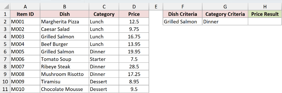
I’ve put the dish I want in cell F2 (Grilled Salmon) and the category in G2 (Dinner). The goal is to return the matching price in H2.
Here is the formula:
=INDEX(D2:D11,MATCH(1,(B2:B11=F2)*(C2:C11=G2),0))
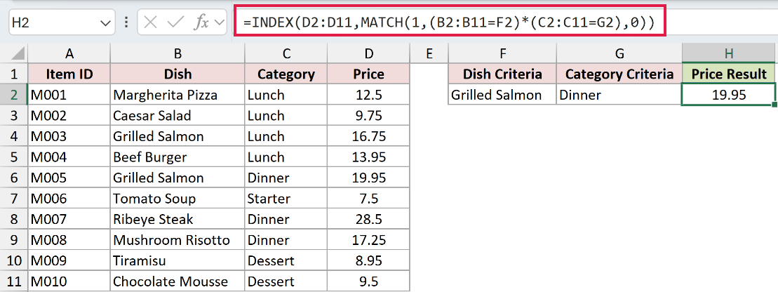
This returns 19.95, the dinner price for Grilled Salmon, not the 16.75 lunch price.
How does this formula work?
(B2:B11=F2) checks every dish against F2 and gives an array of TRUE/FALSE values. (C2:C11=G2) does the same for the category.
Multiplying the two arrays turns them into 1s and 0s. You only get a 1 in the row where both the dish and the category match. Every other row becomes 0.
MATCH(1,...,0) then finds the position of that single 1 in the list. INDEX takes that position and pulls the matching price from column D.
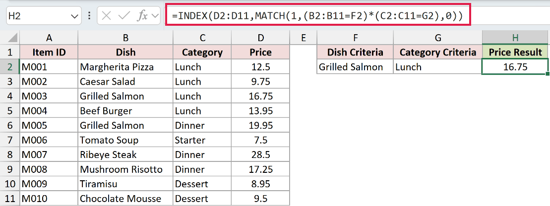
To prove it’s using both conditions, change G2 to Lunch and the result switches to 16.75.
Note: In Excel 365, 2021, or later this works as a normal formula. In Excel 2019 or earlier, press Ctrl+Shift+Enter instead of Enter, or you may get an error or a wrong result. If you’d rather skip that keystroke, use the non-array version in Method #3.
Method #2: Using INDEX MATCH With a Helper Column
If you’d rather avoid array formulas altogether, a helper column keeps things simple. You glue the two criteria columns together into one lookup key, then run an ordinary INDEX MATCH against it.
Here’s the same menu. Grilled Salmon still appears under both Lunch and Dinner, and I want the dinner price in I2.
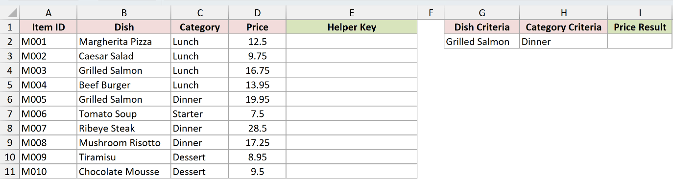
In column E, I’ve built a helper key that joins the dish and category with a pipe character. Enter this in E2 and fill it down to E11:
=B2&"|"&C2
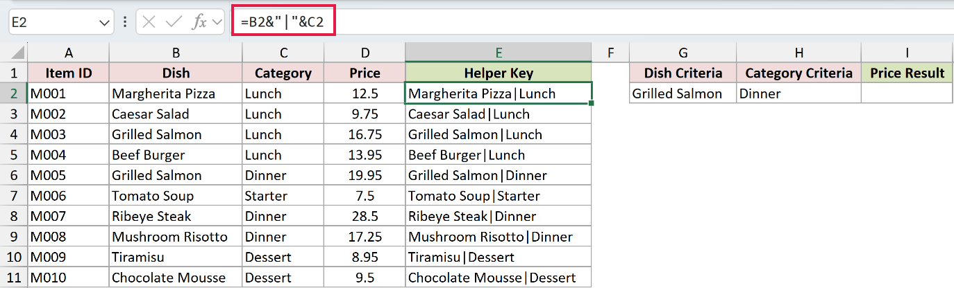
Now E2 reads Margherita Pizza|Lunch, E6 reads Grilled Salmon|Dinner, and so on. Every combination is unique.
Then look up the same joined key with INDEX MATCH:
=INDEX(D2:D11,MATCH(G2&"|"&H2,E2:E11,0))
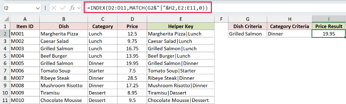
This returns 19.95. MATCH builds the key Grilled Salmon|Dinner from G2 and H2, finds it in the helper column, and INDEX returns the price from column D at that position.
The pipe character matters. It stops values from running together and causing a false match. Without it, a dish ending in a category name could line up with the wrong row.
Note: Pick a delimiter that never appears in your data. A pipe (|) is safe for text like this. If you dislike the extra column, you can hide it once the formula works.
Method #3: Using a Non-Array INDEX MATCH Formula
The array formula in Method #1 works with a plain Enter only in Excel 365 and 2021. In Excel 2019 and earlier you have to press Ctrl+Shift+Enter, and it’s easy to forget. This version wraps the conditions in a second INDEX so it evaluates without any special keystroke, in every version of Excel.
It’s the same menu as before, with the dish in F2 (Grilled Salmon), the category in G2 (Dinner), and the result in H2. Here is the formula:
=INDEX(D2:D11,MATCH(1,INDEX((B2:B11=F2)*(C2:C11=G2),0),0))
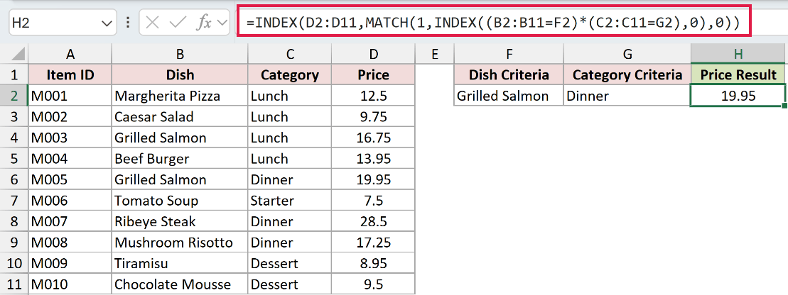
This returns 19.95, the same answer as Method #1, but you press Enter normally.
How does this formula work?
(B2:B11=F2)*(C2:C11=G2) is the same condition trick from Method #1, producing a 1 in the row where both match and a 0 everywhere else. Wrapping it in INDEX(...,0) forces Excel to work out the whole array in one go, which is what an array entry would otherwise do for you.
MATCH(1,...,0) then finds the position of that single 1, and the outer INDEX pulls the price from column D at that row.
Note: The extra INDEX is the whole trick. It lets the formula run with a normal Enter even in Excel 2019 and earlier, so you never have to remember Ctrl+Shift+Enter.
Method #4: Using INDEX MATCH MATCH for Row and Column Criteria
Sometimes your two criteria aren’t two columns in a list. They’re a row heading and a column heading in a grid. INDEX MATCH MATCH is built for this: one MATCH finds the row, the other finds the column, and INDEX returns the value where they cross.
Here the same prices are laid out as a grid. Column A lists each dish, and the Lunch and Dinner prices sit in columns B and C. I’ve put the dish in E2 (Grilled Salmon), the category in F2 (Dinner), and I want the price in G2.
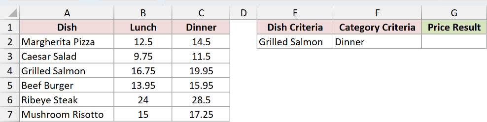
Here is the formula:
=INDEX(B2:C7,MATCH(E2,A2:A7,0),MATCH(F2,B1:C1,0))
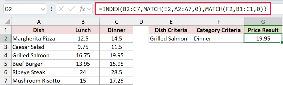
This returns 19.95, the dinner price for Grilled Salmon.
How does this formula work?
MATCH(E2,A2:A7,0) finds which row Grilled Salmon sits on, counting down the dish list. MATCH(F2,B1:C1,0) finds which column Dinner is in, counting across the Lunch and Dinner headers.
INDEX(B2:C7, row, column) then returns the price where that row and column meet. Change the dish or the category and the intersection moves with it.
Note: Reach for INDEX MATCH MATCH whenever your data is a matrix, like products down the side and months across the top. One MATCH per axis and INDEX finds the cell where they meet.
Modern Alternatives: XLOOKUP and FILTER
If you’re on Excel 365 or 2021, two newer functions do the same multi-criteria lookup with less typing. They aren’t INDEX MATCH, but they’re worth having in your back pocket. Both examples use the menu from Method #1, with the dish in F2 and the category in G2.
XLOOKUP joins the criteria with a delimiter right inside the formula, so you skip both the helper column and the array entry:
=XLOOKUP(F2&"|"&G2,B2:B11&"|"&C2:C11,D2:D11,"Not found")
FILTER returns every row that meets both conditions and spills the result. When the combination is unique, that’s a single price:
=FILTER(D2:D11,(B2:B11=F2)*(C2:C11=G2),"Not found")
Both return 19.95. For a fuller look at how XLOOKUP compares, see XLOOKUP Vs INDEX MATCH in Excel and the XLOOKUP Function guide.
Additional Notes About INDEX MATCH with Multiple Criteria in Excel
- Match your ranges. Keep the INDEX or return range (D2:D11) aligned with the criteria ranges. A mismatch can return a value from the wrong row or produce an error.
- Watch for leading or trailing spaces. “Dinner ” with a space won’t equal “Dinner”, and the formula returns no match. Clean the data with TRIM if lookups fail for no obvious reason.
- Text comparisons here are not case sensitive. “grilled salmon” matches “Grilled Salmon”. Use EXACT inside the condition if you need case-sensitive matching.
- More than two criteria is easy. Just add another
*(range=criteria)to the array in Method #1 or Method #3, one for each extra condition.
Frequently Asked Questions
Why does my INDEX MATCH array formula return a #N/A error?
Usually it means no row satisfies both criteria, so check for typos or extra spaces in your criteria cells. It can also happen in Excel 2019 or earlier if you pressed Enter instead of Ctrl+Shift+Enter.
How do I do INDEX MATCH with multiple criteria without Ctrl+Shift+Enter?
In Excel 365 or 2021 the array formula in Method #1 already works with a plain Enter. In older versions, use the non-array formula in Method #3, which nests an extra INDEX so it runs without the special keystroke.
Can INDEX MATCH with multiple criteria return more than one match?
No. INDEX MATCH returns only the first matching row. If you need every matching row, use the FILTER function from the alternatives above, which spills all of them.
Do I need to enter the array formula with Ctrl+Shift+Enter?
Only in Excel 2019 and earlier. In Excel 365, Excel 2021, and later, the formula in Method #1 works with a normal Enter because dynamic arrays handle it automatically.
Conclusion
You now have four ways to run an INDEX MATCH with multiple criteria in Excel. The array formula in Method #1 is my default because it needs no helper column.
If you’re on Excel 2019 or earlier, the non-array version in Method #3 saves you the Ctrl+Shift+Enter. And when your data is laid out as a grid, INDEX MATCH MATCH in Method #4 is the one to reach for.
If you’re on Excel 365 or 2021 and want something shorter, XLOOKUP and FILTER get you there too. Pick the one that fits your version, and you’ll never grab the wrong price again.
Other Excel articles you may also like:
