If you want to clean up text in Excel that has extra spaces at the start, end, or between words, the TRIM function is what you’re looking for.
In this article, I’ll show you how to use TRIM in Excel with a few practical examples, plus the one type of space it cannot remove on its own.
In Excel 365, you can also feed TRIM a whole range and the cleaned values will spill into the cells below as a single formula. No more dragging the formula down a helper column.
TRIM Function Syntax
Here is the syntax of the TRIM function:
=TRIM(text)
- text – The text string (or a cell reference) you want to clean up. In Excel 365 and 2021, this can also be a whole range — the cleaned values will spill across the cells below your formula.
When to Use TRIM Function in Excel
Use this function when you need to:
- Remove leading and trailing spaces from text typed by users or imported from another system.
- Collapse multiple spaces between words down to a single space.
- Clean up a whole column of imported text in one go (Excel 365 spills the result automatically).
- Clean up data before using it in lookups like VLOOKUP or XLOOKUP, where stray spaces silently break matches and leave you wondering why your VLOOKUP is not working.
Let me show you a few practical examples of how TRIM works.
Example 1: Spill Cleaned Text Across a Whole Column
Let’s start with the most common use case.
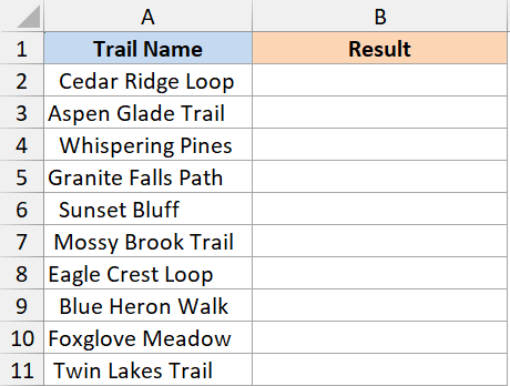
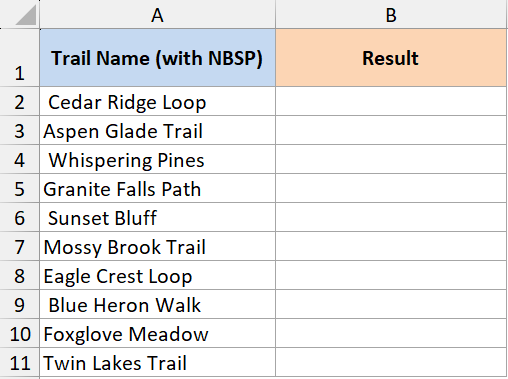
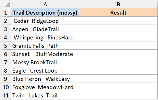
Below is a list of hiking trail names exported from a state park database.
The CSV came in with extra spaces before and after the actual names. You cannot tell just by looking at the cells, but a lookup against this list would silently fail because of those hidden spaces.
I want a clean column of trail names with the stray spaces gone.
Here is the formula:
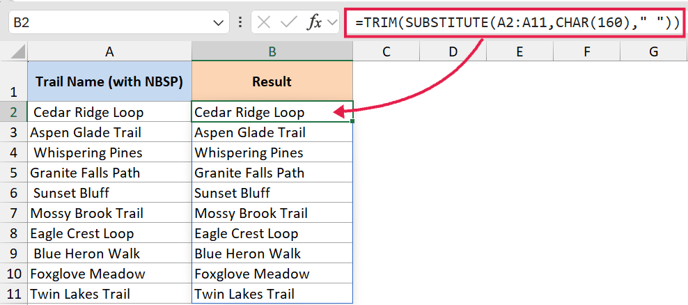
=TRIM(A2:A11)
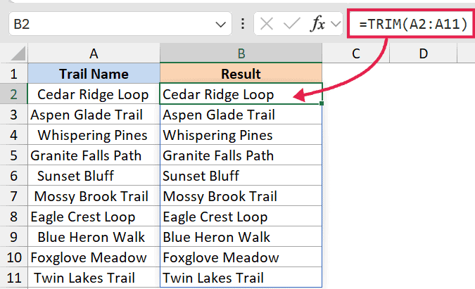
In the above formula, TRIM looks at every cell in the range A2:A11, strips out every space before the first word and every space after the last word, and spills the cleaned values into B2:B11 as a single formula. No drag-down, no helper column to copy.
If you want to overwrite the original list, copy the spilled output and paste it back as values over the original cells.
For more cleanup techniques specific to the start of a string, see this guide on how to remove leading spaces in Excel.
Example 2: Collapse Multiple Spaces Between Words
Here’s another scenario you’ll run into often.
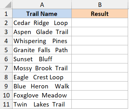
Sometimes data comes in with two or three spaces between words instead of one, usually because someone typed it that way or it got pulled from a system that handled spacing oddly.
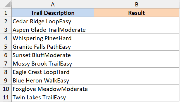
The same trail database in this example has descriptions where the spacing is all over the place.
Here is the formula:
=TRIM(A2:A11)
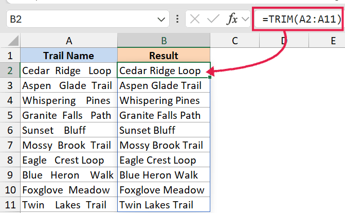
What happens is TRIM collapses any run of two or more spaces between words down to a single space.
It leaves exactly one space between words intact, so the sentence still reads naturally. The spill operator means one formula handles the whole column at once.
So "Cedar Ridge Loop" becomes "Cedar Ridge Loop". No need for Find and Replace, no manual cleanup. If you specifically need to remove space before text, TRIM handles that case too.
Example 3: What TRIM Does NOT Remove
Now for the gotcha that trips a lot of people up.
If you copy text from a website or paste from a Word document, the “spaces” in that text are often not regular spaces.
They are non-breaking spaces, which Excel sees as character 160 (CHAR(160)) instead of the regular space, which is character 32.
TRIM only removes character 32. So you’ll run TRIM, the cell will still look like it has weird spaces, and you’ll wonder what’s going on.
Here is the formula that handles it:
=TRIM(SUBSTITUTE(A2:A11,CHAR(160)," "))
How this formula works:
- SUBSTITUTE(A2:A11, CHAR(160), ” “) first replaces every non-breaking space across the whole range with a regular space.
- TRIM(…) then runs on the cleaned-up array and strips the leading, trailing, and duplicate spaces the normal way.
- The result spills into the cells below your formula, one cleaned value per source row.
This combo is the one I reach for whenever I deal with text that came from a web page, a PDF, or a corporate report. The same SUBSTITUTE plus TRIM pattern also shows up in tricks like how to extract the last word in a cell.
Example 4: TRIM and CLEAN Combo for Line Breaks
Here’s another case that comes up with imported data.
Some text doesn’t just have weird spaces. It also has invisible non-printing characters, like line breaks, tabs, or other control characters that snuck in from the source system. TRIM can’t touch those either.
That’s where the CLEAN function comes in. CLEAN strips out the first 32 non-printing characters in the ASCII set, which includes most of the junk you’ll encounter.
Here is the formula:
=TRIM(CLEAN(A2:A11))
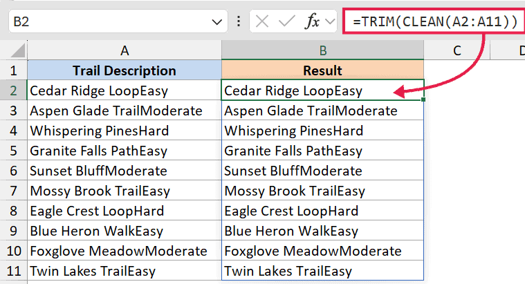
In the above formula, CLEAN runs first across the whole range and pulls out line breaks and other non-printing junk. TRIM then cleans up the spaces that get left behind.
Together, they handle most messy text in a single spilling formula.
Example 5: The Full Data Cleanup Combo
If you really want to bulletproof your text cleanup, stack all three together.
This handles regular spaces, non-breaking spaces, and non-printing characters in one shot. Use this when you have no idea where the data came from and just need it cleaned.
Here is the formula:
=TRIM(CLEAN(SUBSTITUTE(A2:A11,CHAR(160)," ")))
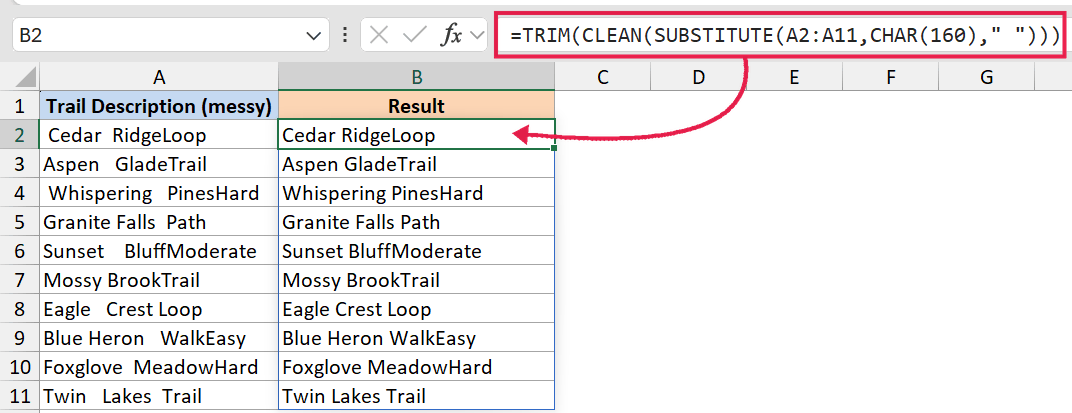
How this formula works:
- SUBSTITUTE swaps non-breaking spaces (CHAR(160)) for regular spaces across every row in the range.
- CLEAN removes line breaks, tabs, and other non-printing characters from each row.
- TRIM finishes the job by trimming leading, trailing, and duplicate spaces.
- The whole thing spills as one formula, so you get a fully cleaned column from a single cell.
This is my go-to formula for any data import where I don’t trust the source. Drop it next to your messy column, copy the spilled result, and paste back as values.
Tips & Common Mistakes
- TRIM only handles regular spaces (CHAR(32)). If the cell still looks dirty after running TRIM, the culprit is almost always non-breaking spaces (CHAR(160)). Wrap the range in SUBSTITUTE first.
- TRIM converts numbers to text. If you run TRIM on a number, the result is a text string. If you need it back as a number, multiply by 1 or wrap the result in VALUE().
- Lookup failures are often a TRIM problem. If VLOOKUP or XLOOKUP returns #N/A and the values look identical, run TRIM on both sides before troubleshooting anything else.
#SPILL!means the spill range is blocked. If you write=TRIM(A2:A100)and one of the cells below already has data, Excel can’t lay down the spilled result. Clear the spill range, or move the formula somewhere with empty cells underneath.- Watch out for the
@implicit intersection. A workbook saved by an older Excel version sometimes auto-injects an@symbol (e.g.=@TRIM(A2:A100)), which collapses the spill back to a single cell. Remove the@and the spill comes back. - Use Find and Replace for one-off cleanup. If you only need to clean a small range, Ctrl+H to replace double spaces with single spaces is faster than writing a formula. TRIM is for repeatable, formula-driven cleanup.
- Don’t forget to paste as values. TRIM gives you a formula result. To replace the original messy column, copy the TRIM output and paste over the original as values, then delete the helper column.
That covers the main ways to use TRIM in Excel. Once you get comfortable feeding TRIM a whole range and wrapping it with SUBSTITUTE and CLEAN, most text-cleaning problems become a one-formula job.
Related Excel Functions / Articles:
- UPPER Function in Excel
- How to Remove a Specific Character from a String in Excel
- How to Extract Text After Space Character in Excel?
- How to Remove Question Marks from Text in Excel?
- Bulk Find and Replace in Excel
- Remove the Last 4 Characters in Excel
- Opposite of Concatenate in Excel (Reverse Concatenate)
- How to Remove Numbers From Text in Excel