
INDEX MATCH is a lookup combo, but MATCH only ever finds the first row that matches. So if a value appears several times, you only get one result back.
To pull every matching value, you keep INDEX and swap MATCH for something that can return the 2nd, 3rd, and 4th match too. That’s what the formulas below do.
For example, you can list every attendee signed up for one workshop, either down a column or joined into a single cell.
In this article, I’ll show you how to return all matches with INDEX and SMALL, INDEX and AGGREGATE, TEXTJOIN, and the FILTER function.
Method #1: Using INDEX, SMALL, and IF
This is the classic way to return multiple values with INDEX. It works in every Excel version, which makes it handy if you share files with people on older Excel.
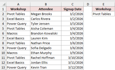
Below I have a dataset of workshop signups, with workshops in column A and attendees in column B. I want every attendee for the workshop in cell E2.
Here is the formula to enter in cell G2:
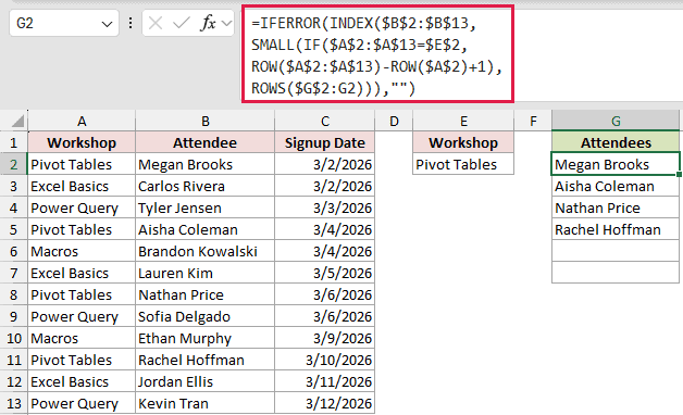
=IFERROR(INDEX($B$2:$B$13,SMALL(IF($A$2:$A$13=$E$2,ROW($A$2:$A$13)-ROW($A$2)+1),ROWS($G$2:G2))),"")
Then copy it down to G7. The four Pivot Tables attendees show up in G2:G5, and the extra cells stay blank.
How does this formula work?
$A$2:$A$13=$E$2 checks each workshop against Pivot Tables and returns an array of TRUE and FALSE values.
ROW($A$2:$A$13)-ROW($A$2)+1 turns the rows into positions 1 to 12. IF keeps the position for each TRUE and returns FALSE for everything else.
ROWS($G$2:G2) is a counter. It returns 1 in G2, 2 in G3, and so on, because the range grows by one row each time you copy the formula down.
SMALL uses that counter to pick the 1st, 2nd, 3rd smallest position. INDEX then returns the attendee name from column B at that position.
Once the counter goes past the number of matches, SMALL returns a #NUM! error. IFERROR catches that and shows a blank instead.
Note: In Excel 2019 and earlier versions, this is an array formula. Enter it with Ctrl + Shift + Enter instead of just Enter, then copy it down. In Microsoft 365 and Excel 2021, a regular Enter works.
Method #2: Using INDEX and AGGREGATE (Recommended)
This is the method I’d recommend for most people. It does the same job as Method #1, but you never have to enter it with Ctrl + Shift + Enter.
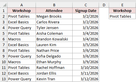
Below I have the same workshop signup dataset. Again, I want every attendee for the workshop in cell E2.
Here is the formula to enter in cell G2:
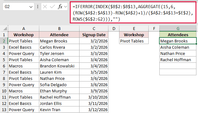
=IFERROR(INDEX($B$2:$B$13,AGGREGATE(15,6,(ROW($A$2:$A$13)-ROW($A$2)+1)/($A$2:$A$13=$E$2),ROWS($G$2:G2))),"")
Copy it down to G7. You get Megan Brooks, Aisha Coleman, Nathan Price, and Rachel Hoffman, with blanks below them.
How does this formula work?
AGGREGATE can run several functions. The first argument, 15, tells it to act like SMALL. The second argument, 6, tells it to ignore error values.
(ROW($A$2:$A$13)-ROW($A$2)+1) gives the positions 1 to 12. Dividing them by ($A$2:$A$13=$E$2) does the real work here.
A matching row divides by TRUE (which Excel treats as 1), so the position stays as it is. A non-matching row divides by FALSE (0) and returns a #DIV/0! error.
Since option 6 skips errors, AGGREGATE only sees the positions of the Pivot Tables rows. ROWS($G$2:G2) picks the 1st, 2nd, 3rd of them as you copy down.
INDEX returns the attendee at each position, and IFERROR shows a blank once there are no more matches.
Method #3: Using the TEXTJOIN Function
If you’d rather have all the matches in one cell, TEXTJOIN is the way to go. It joins every matching value into a single list separated by commas.
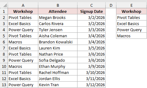
Below I have the same dataset, and this time I’ve listed four workshops in column E. I want all the attendees for each workshop next to it in column F.
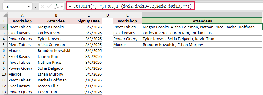
Here is the formula to enter in cell F2:
=TEXTJOIN(", ",TRUE,IF($A$2:$A$13=E2,$B$2:$B$13,""))
Copy it down to F5. For Pivot Tables, you get “Megan Brooks, Aisha Coleman, Nathan Price, Rachel Hoffman” in one cell.
How does this formula work?
IF checks each workshop in A2:A13 against E2. For a match, it returns the attendee name from column B. For everything else, it returns an empty text string.
TEXTJOIN then joins that list with a comma and a space. The TRUE argument tells it to skip the empty strings, so you don’t get extra commas.
I left E2 as a relative reference, so it changes to E3, E4, and E5 as you copy the formula down. The data ranges are locked with dollar signs.
Note: TEXTJOIN is available in Excel 2019 and later. In Excel 2019, you may need to confirm this formula with Ctrl + Shift + Enter because of the IF array inside it.
Method #4: Using the FILTER Function
If you have Microsoft 365 or Excel 2021, the FILTER function is the simplest option. One formula returns all the matches, and you don’t copy anything down.
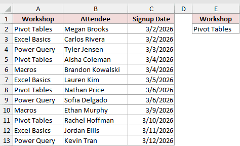
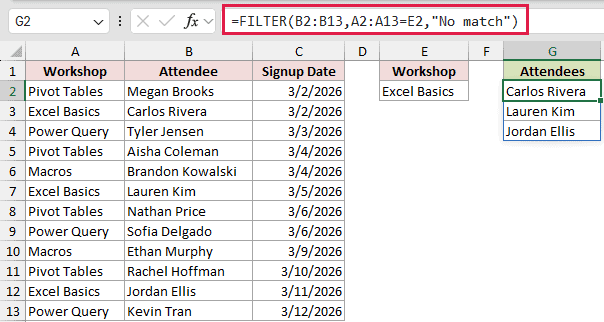
Below I have the same workshop signup dataset. I want every attendee for the workshop in cell E2.
Here is the formula to enter in cell G2:
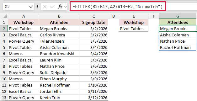
=FILTER(B2:B13,A2:A13=E2,"No match")
How does this formula work?
FILTER returns the values from B2:B13 wherever A2:A13 equals the workshop in E2. The four Pivot Tables attendees spill into G2:G5 automatically.
The third argument, “No match”, is what FILTER returns when nothing matches. Without it, you’d get a #CALC! error for a workshop with no signups.
The result also resizes on its own. If I change E2 to Excel Basics, the list shrinks to Carlos Rivera, Lauren Kim, and Jordan Ellis.
Note: Keep the cells below G2 empty. If anything blocks the spill range, FILTER returns a #SPILL! error instead of the names.
Additional Notes About Returning Multiple Values With INDEX MATCH
- MATCH on its own can’t return more than one row. If you only need the first match, a regular INDEX MATCH is fine. The methods above are for getting every match.
- In Methods #1 and #2, copy the formula down to more rows than you expect to need. Extra rows stay blank, but too few rows quietly cut off matches.
- Lock the data ranges with dollar signs in the copy-down formulas. Otherwise, the ranges shift as you copy and you start missing rows.
- All four methods are exact matches, and none of them are case-sensitive. “pivot tables” in E2 still returns the same four names.
Frequently Asked Questions
Can INDEX MATCH Return Multiple Values in Excel?
Not with MATCH alone, since MATCH stops at the first match. You need to replace MATCH with SMALL(IF()) or AGGREGATE, which return the position of each match in turn.
How Do I Return Multiple Values Horizontally Instead of Vertically?
In Methods #1 and #2, replace ROWS($G$2:G2) with COLUMNS($G$2:G2) and copy the formula to the right. With FILTER, wrap it in TRANSPOSE to spill across a row.
How Do I Return Multiple Values Based on Multiple Criteria?
With FILTER, multiply the conditions together. For example, (A2:A13=E2)*(C2:C13=F2) returns only the rows where both conditions are true.
Why Does My Formula Show #NUM! After the Last Match?
That happens in Methods #1 and #2 when there are no more matches to return. Wrapping the formula in IFERROR, as shown above, turns those errors into blanks.
Conclusion
In this article, I showed you four ways to return multiple values with INDEX and its alternatives: INDEX with SMALL and IF, INDEX with AGGREGATE, TEXTJOIN, and FILTER.
If you have Microsoft 365, FILTER is the quickest. For older Excel versions where you would rather skip Ctrl + Shift + Enter, go with INDEX and AGGREGATE.
I hope you found this article helpful.
Other Excel articles you may also like:
- INDEX MATCH with Multiple Criteria in Excel
- How to Use VLOOKUP with Multiple Criteria in Excel
- XLOOKUP Vs INDEX MATCH in Excel
- MATCH Function in Excel
- Find the Row Number of Matching Value in Excel
- Find Last Occurrence of a Value in a Column in Excel
- XLOOKUP Function in Excel
- Extract Unique Values Based on Conditions in Excel
