
If you want to measure how closely two sets of numbers move together, the CORREL function returns their Pearson correlation coefficient.
In this article, I’ll show you how to interpret positive and negative results, handle incomplete data, calculate a group-specific correlation, and compare several drivers at once.
CORREL returns one value from two arrays, but it also works inside dynamic array formulas such as =CORREL(FILTER(...),FILTER(...)).
CORREL Function Syntax in Excel
Here is the syntax of the CORREL function:
=CORREL(array1, array2)
array1is the first range of numeric observations. This argument is required.array2is the second range of numeric observations. This argument is required.
The result ranges from -1 to 1. Values closer to 1 indicate a stronger positive linear relationship, while values closer to -1 indicate a stronger negative linear relationship. A result near 0 indicates a weak or absent linear relationship.
The two arrays must represent paired observations and contain the same number of data points. CORREL measures association, but it does not show that one variable causes the other.
For a wider look at Excel’s other methods, see my guide to calculating a correlation coefficient in Excel.
When to Use CORREL Function
Use CORREL when you need to:
- Measure whether two numeric variables tend to rise together.
- Check whether one variable tends to fall as another rises.
- Compare operational measures recorded for the same periods or subjects.
- Calculate a correlation for one category or group.
- Compare several possible drivers with one outcome.
Example 1: Measure a Positive Correlation
I’ll begin with two measures that generally rise together.
The dataset below contains weekly demo requests in column B and new contracts in column C.
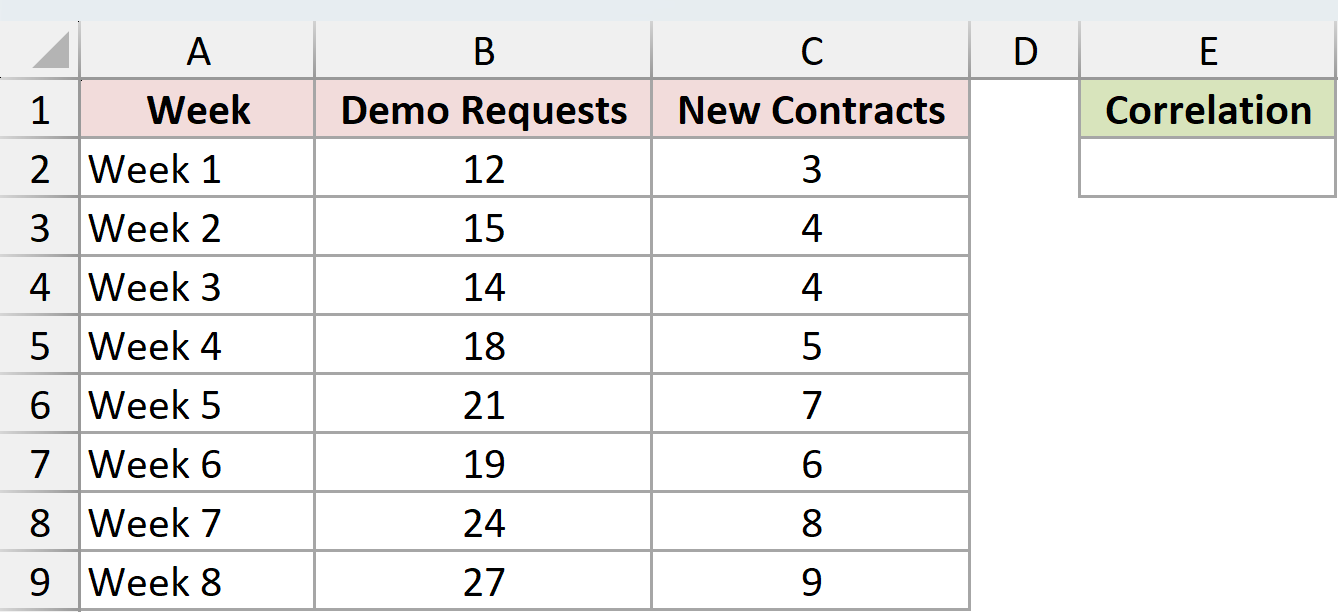
I want to measure the linear relationship between demo requests and new contracts.
Here is the formula:
=CORREL(B2:B9,C2:C9)
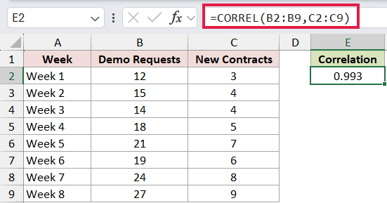
CORREL pairs each week’s value in column B with the contract count from the same row in column C. The formula returns 0.993 when rounded to three decimal places.
That result is close to 1, so this small dataset has a strong positive linear relationship. Weeks with more demo requests generally had more new contracts.
The PEARSON function returns the same Pearson correlation coefficient. CORREL is usually the easier name to recognize in a worksheet.
Pro Tip: A high coefficient does not prove that demo requests caused the contracts. CORREL measures how the values move together, not why they moved.
If you only need to check two short lists, you can also use this correlation coefficient calculator.
Example 2: Measure a Negative Correlation
Now consider two measures that move in opposite directions.
This warehouse dataset pairs each shift’s average pick distance with the number of items picked per hour.
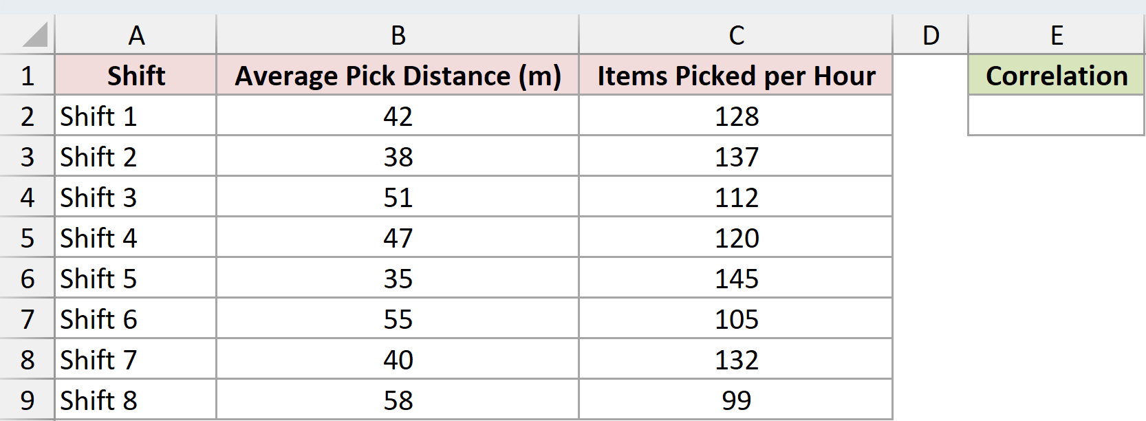
I want to see whether longer pick distances are associated with lower throughput.
Here is the formula:
=CORREL(B2:B9,C2:C9)
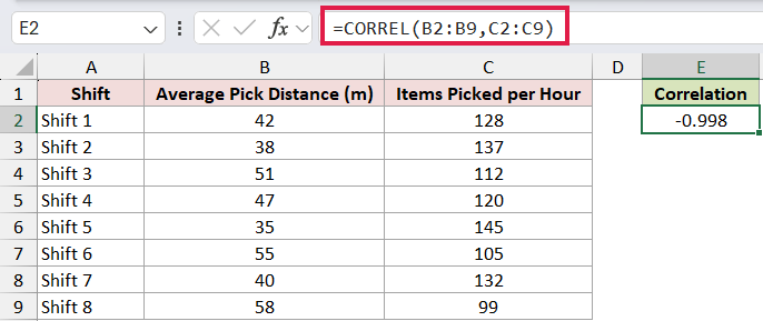
The result is -0.998 when rounded to three decimal places. It is close to -1, which indicates a strong negative linear relationship in these eight shifts.
As pick distance increases, items picked per hour generally decreases. The negative sign describes the direction of the relationship. It does not mean the formula or data is wrong.
I recommend pairing CORREL with a scatter plot when you need to inspect outliers or a curved pattern.
You can also add a trendline to make the overall direction easier to see.
Example 3: Handle Blanks, Text, and Zeros
Operational datasets often contain unfinished rows and status text.
This test log records valve opening percentages and flow rates. It includes a paired blank row, a paired Pending row, and a valid zero reading.
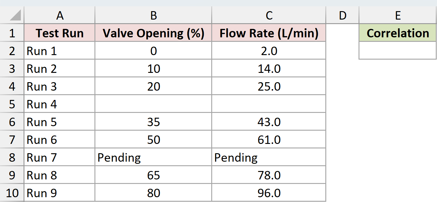
I want to calculate the correlation from the usable numeric observations.
Here is the formula:
=CORREL(B2:B10,C2:C10)
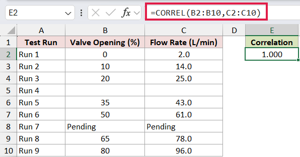
CORREL ignores the paired blank cells and the paired text entries. It includes the zeros in row 2 because zero is a numeric observation.
The underlying result is about 0.999966. The result cell displays 1.000 because its number format shows only three decimal places, but the relationship is not mathematically perfect.
Pro Tip: Display more decimal places before treating a rounded result as exactly 1 or -1. Cell formatting can hide a small difference.
Example 4: Calculate Correlation for One Group
You do not need helper columns to calculate a coefficient for one category.
The dataset below contains queue lengths and wait times for Downtown and Airport branches. Cell E2 contains the branch I want to analyze.
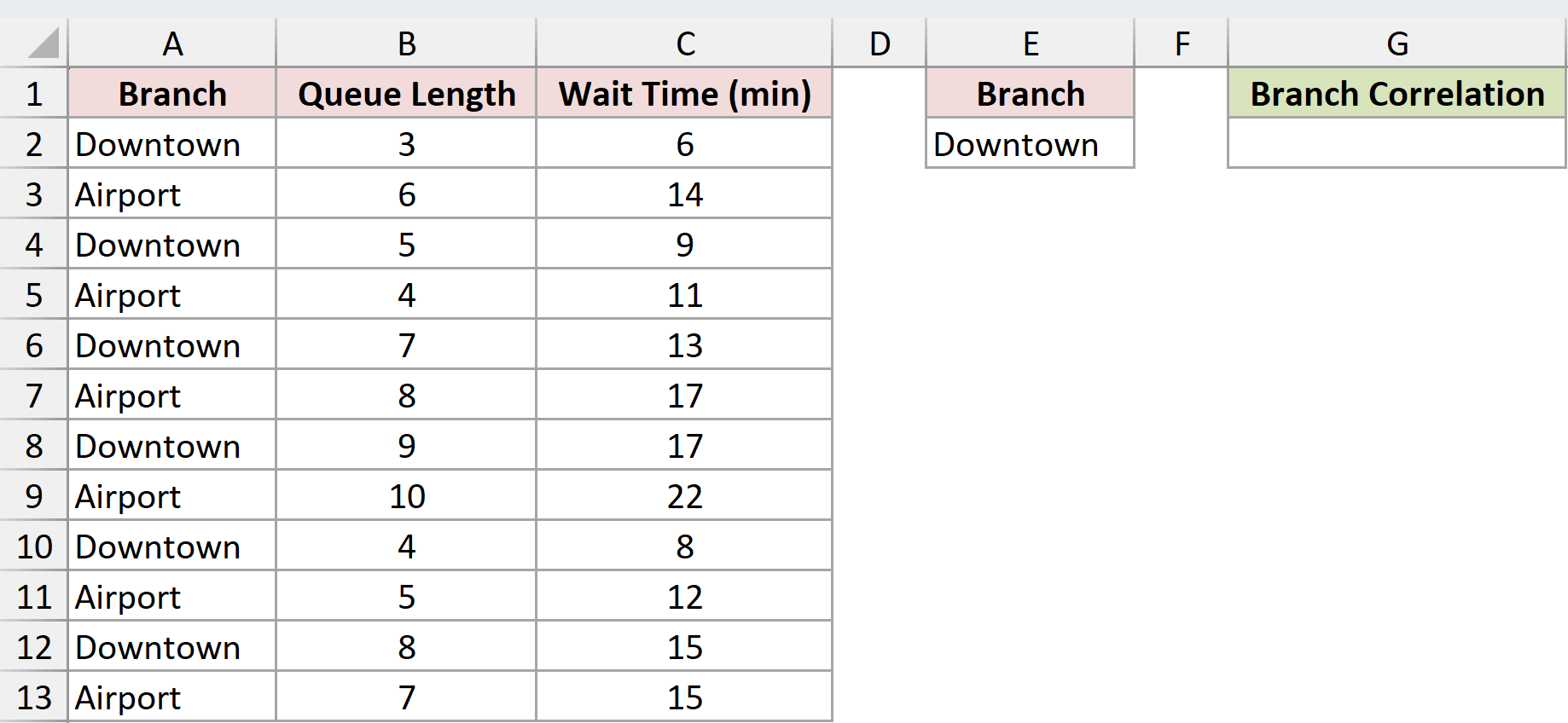
I want the correlation between queue length and wait time for Downtown rows only.
Here is the formula:
=CORREL(FILTER(B2:B13,A2:A13=E2),FILTER(C2:C13,A2:A13=E2))
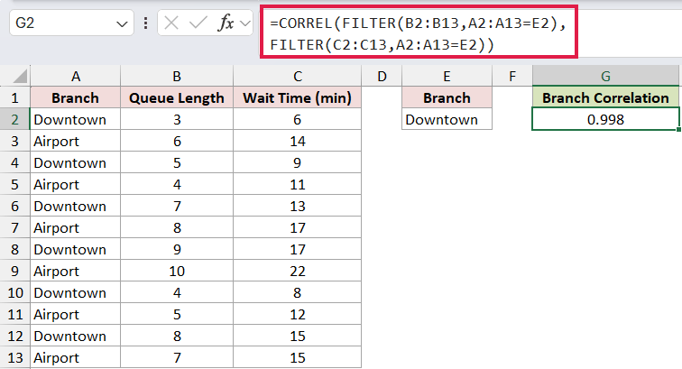
How this formula works:
- The first FILTER function returns the queue lengths for the branch in E2.
- The second FILTER returns wait times using the same branch test.
- CORREL calculates the coefficient from those two filtered arrays.
With Downtown in E2, the formula returns 0.998 when rounded to three decimal places. Change E2 to Airport and both arrays update from the same set of rows.
FILTER is available in Microsoft 365, Excel 2024, and Excel 2021.
Pro Tip: Both FILTER calls must use the same condition. If the arrays represent different rows or contain different numbers of data points, the coefficient will not describe valid pairs.
Example 5: Compare Several Drivers at Once
CORREL normally reduces two arrays to one coefficient, but BYCOL can repeat that calculation across several columns.
This weekly funnel dataset has webinar registrations, demo bookings, and trial activations in columns B:D. New contracts are in column E.
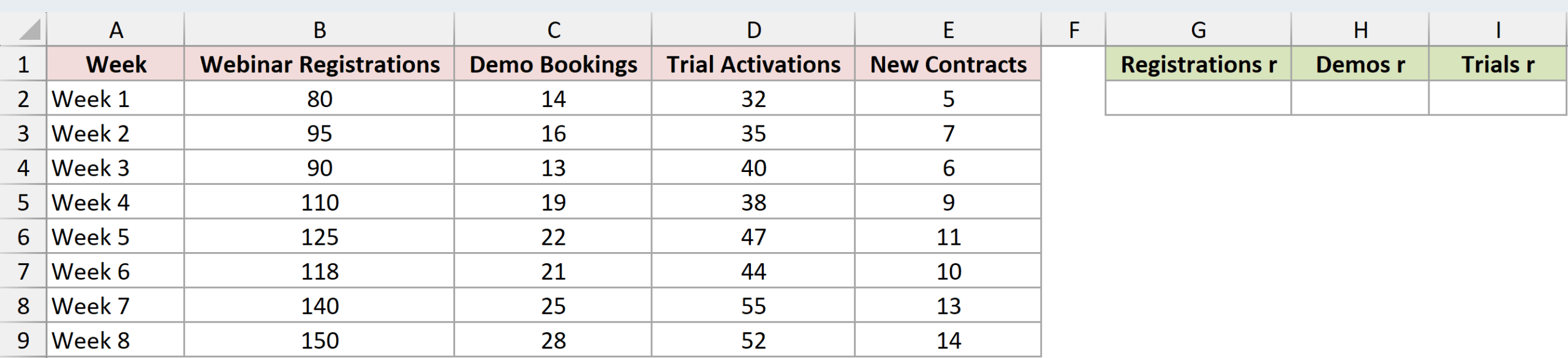
I want one correlation coefficient for each activity column compared with new contracts.
Here is the formula:
=BYCOL(B2:D9,LAMBDA(activity,CORREL(activity,E2:E9)))
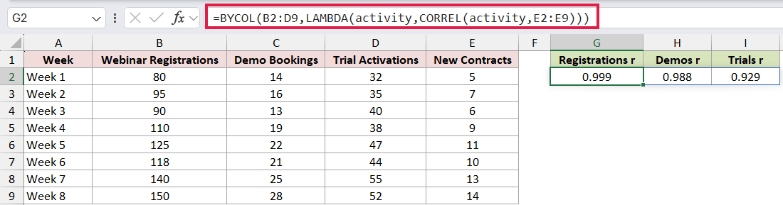
How this formula works:
- BYCOL passes one column from B2:D9 to the LAMBDA at a time.
activityis the temporary name for the current activity column.- CORREL compares that column with the new-contract range E2:E9.
The formula spills three results across G2:I2. Registrations returns 0.999, demos returns 0.988, and trials returns 0.929 when displayed to three decimal places.
BYCOL and LAMBDA are available in Microsoft 365 and Excel 2024. For a large correlation matrix, Excel’s Correlation tool in the Analysis ToolPak is usually more convenient.
Tips & Common Mistakes
- CORREL requires paired arrays with the same number of data points. Different lengths return a #N/A error.
- Text, logical values, and blank cells in referenced arrays are ignored. Zero values remain part of the calculation.
- CORREL returns #DIV/0! if either usable array is empty or has no variation.
- A result near 0 means little or no linear relationship. The data may still have a nonlinear pattern, so inspect a chart when that possibility matters.
- Correlation does not establish cause and effect. Treat the coefficient as one part of the analysis rather than a conclusion by itself.
- CORREL returns one coefficient by itself. Use FILTER for a selected group or BYCOL with LAMBDA when you need a dynamic array composition.
I covered positive and negative correlation, ignored values, group-specific analysis, and a multi-column comparison. I hope you found this article helpful.
Related Excel Functions / Articles:
