
If you want to join separate ranges side by side without copying columns, the HSTACK function is built for the job.
You’ll learn how to build cleaner horizontal arrays with HSTACK.
HSTACK is a dynamic array function. It spills its results across the cells to the right and below.
HSTACK Function Syntax in Excel
The HSTACK function accepts two or more arrays and places each one to the right of the previous array.
=HSTACK(array1,[array2],...)
- array1 (required) is the first array or range you want in the combined result.
- array2 (optional) is the next array or range to place beside the first. You can add more arrays as needed.
The result has the combined width of all supplied arrays. Its height matches the tallest array.
When to Use HSTACK Function
- Join columns from separate ranges without copying and pasting them into a new table.
- Place related lists beside each other, even when the lists contain different numbers of rows.
- Add a generated index or calculated column to an existing array.
- Select non-adjacent columns before filtering or sorting the result.
Example 1: Combine Two Ranges Side by Side
Let’s start by rebuilding a full-year sales table from two separate blocks.
Below is the dataset. Columns A to C contain each store’s Q1 and Q2 sales. Columns E and F contain Q3 and Q4 sales.
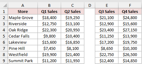
We want to combine both blocks into one five-column table beginning in H2.
Here is the formula:
=HSTACK(A2:C9,E2:F9)
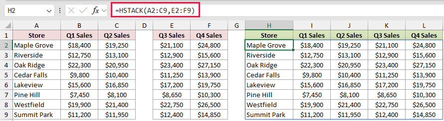
HSTACK takes all three columns from A2:C9, then places the two columns from E2:F9 immediately to their right.
The single formula returns eight rows and five columns. Maple Grove’s row, for example, shows sales of $18,400, $19,250, $21,100, and $24,800.
When all required columns sit inside one continuous source range, CHOOSECOLS can also select them. HSTACK is more flexible when the blocks come from separate ranges.
Pro Tip: Keep the entire output area empty before entering the formula. A value in any destination cell blocks the result and causes a #SPILL! error.
Example 2: Handle Unequal Lists and #N/A
Here’s what happens when the ranges aren’t the same height.
Below is the dataset. Column A lists seven morning-shift employees, while column C lists five evening-shift employees.
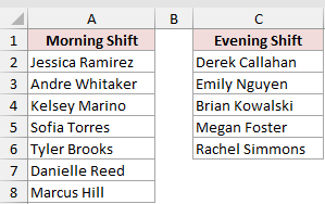
We want to place the two shift lists beside each other and then remove the padding errors.
Here is the basic HSTACK formula:
=HSTACK(A2:A8,C2:C6)
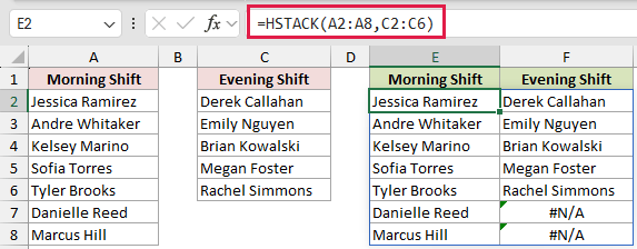
The result is seven rows tall because A2:A8 is the taller array. Excel fills the final two cells in the shorter evening column with #N/A.
To display those padding cells as empty, wrap HSTACK in IFNA:
=IFNA(HSTACK(A2:A8,C2:C6),"")
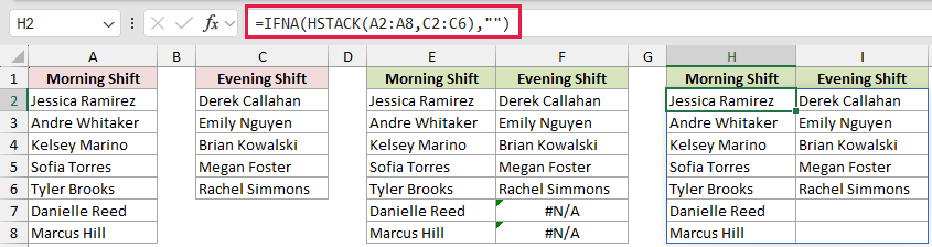
IFNA replaces only the #N/A values with empty text. The five names in the evening list and all seven morning names stay unchanged.
You could also use EXPAND to pad the shorter list before stacking it. IFNA is easier when you only need to clean the final output.
Pro Tip: The "" returned by IFNA is an empty text string, not a truly blank cell. This distinction can matter when another formula counts or tests the output.
Example 3: Add an Index Column With SEQUENCE
Running numbers are easy to add without creating a helper column.
Below is the dataset. Columns A and B contain ten tasks and their owners.
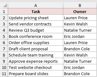
We want to place the numbers 1 through 10 before the task list.
Here is the formula:
=HSTACK(SEQUENCE(ROWS(A2:A11)),A2:B11)
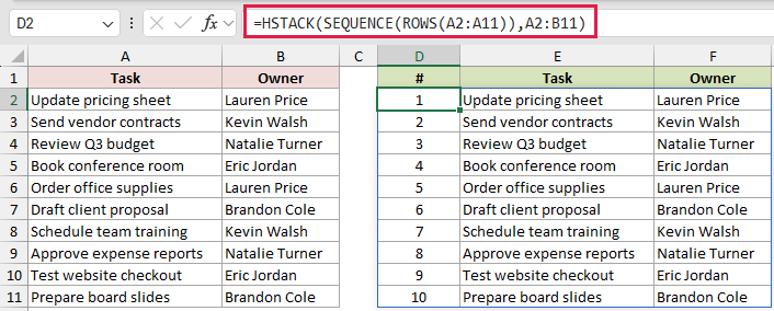
ROWS counts the ten task rows. SEQUENCE creates a vertical array from 1 to 10, and HSTACK places that array before columns A and B.
Because the number of generated values comes from ROWS, the index and task ranges stay the same height.
This approach avoids a helper column filled with row-number formulas. It also keeps the source task list untouched.
Example 4: Append a Calculated Column
An array calculation can also serve as an HSTACK input.
Below is the dataset. Columns A to C contain office items, quantities, and unit prices.
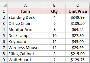
We want to copy the three source columns and append each item’s line total.
Here is the formula:
=HSTACK(A2:C9,B2:B9*C2:C9)
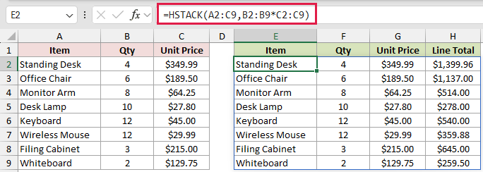
The expression B2:B9*C2:C9 multiplies each quantity by its matching unit price. HSTACK appends the eight calculated values as a fourth column.
For example, four standing desks at $349.99 produce a line total of $1,399.96. Twelve wireless mice at $29.99 produce $359.88.
Pro Tip: HSTACK returns values, not the source cell formatting. Apply currency formatting to the spill output separately.
Example 5: Build a Filtered and Sorted Report
Finally, let’s combine HSTACK with FILTER and SORT to create a small report.
Below is the dataset. Columns A to D contain order IDs, customers, statuses, and amounts.
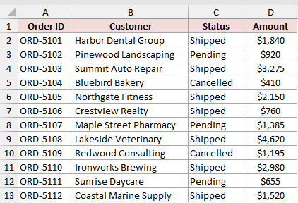
We want a two-column report of shipped customers, ordered from the highest amount to the lowest.
Here is the formula:
=SORT(FILTER(HSTACK(B2:B13,D2:D13),C2:C13="Shipped"),2,-1)
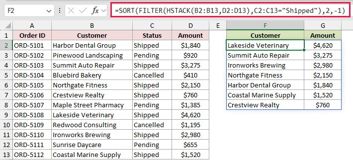
HSTACK first joins the Customer and Amount columns. FILTER keeps the seven rows where the Status column contains Shipped.
SORT then uses column 2 of the stacked array and a sort order of -1. This places the largest amount first.
Lakeside Veterinary appears at the top with $4,620. Crestview Realty appears last with $760.
Because both selected columns come from one table, CHOOSECOLS can replace HSTACK here.
Tips & Common Mistakes
- HSTACK is available in Microsoft 365 and Excel 2024 or later. Older Excel versions return #NAME? for this function.
- The output needs enough empty cells to the right and below the formula. Clear anything blocking that area if Excel returns #SPILL!.
- Shorter arrays receive #N/A padding. Use IFNA when you want to hide only those errors, rather than IFERROR, which hides every error type.
- HSTACK can accept many arrays. Separate each array with the list separator used by your regional Excel settings.
- A spill reference such as
H2#refers to the full HSTACK result and expands or contracts with it. - Use VSTACK when you need to place arrays below one another instead of side by side.
HSTACK gives you one formula for combining ranges horizontally, with no helper table to maintain.
Once the basic side-by-side join makes sense, you can shape the spilled output for more demanding reports.
Related Excel Functions / Articles:
