
If you want a smaller view of a wide table, CHOOSECOLS lets you pull out the columns you need without copying them elsewhere.
In this article, I’ll show you how to select, reorder, and combine columns using practical CHOOSECOLS formulas.
CHOOSECOLS is a dynamic array function. You enter it in one cell, and the selected columns spill into the cells to the right and below.
CHOOSECOLS Function Syntax in Excel
The CHOOSECOLS function takes an array and returns the columns identified by one or more column numbers.
=CHOOSECOLS(array, col_num1, [col_num2], ...)
- array (required) is the range or array containing the columns you want to return.
- col_num1 (required) identifies the first column to return.
- col_num2 (optional) identifies another column to return. You can add more column numbers as needed.
- Positive column numbers count from the left. Negative column numbers count from the right.
When to Use CHOOSECOLS Function
- Create a smaller view of a wide export without changing the source table.
- Return nonadjacent columns in one spilled result.
- Rearrange columns into a different order.
- Select columns from the right without counting every source column.
- Combine CHOOSECOLS with FILTER, XMATCH, and HSTACK to filter rows or generate arrays of column positions.
Example 1: Select Nonadjacent Columns from a Table
Let’s start with the most common use of CHOOSECOLS.
Below is the dataset. Columns A through F contain ten veterinary visits, including visit IDs, pets, species, owners, dates, and fees.
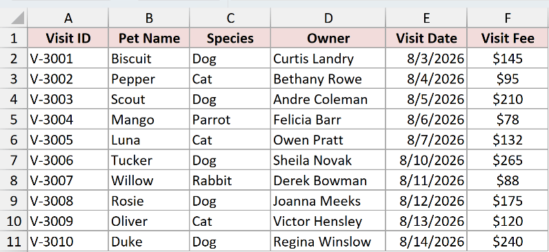
We want to return the Pet Name, Owner, and Visit Fee columns in H2:J11.
Here is the formula:
=CHOOSECOLS(A2:F11,2,4,6)
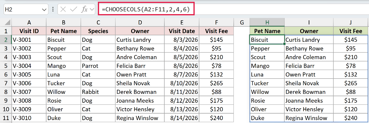
The numbers 2, 4, and 6 tell Excel which source columns to return. The output order follows that same argument order.
The first result row contains Biscuit, Curtis Landry, and $145. The last contains Duke, Regina Winslow, and $240.
Because the array starts at A2, the source headers are not included. The three headers in H1:J1 were entered separately.
Example 2: Rearrange Columns in Any Order
Here’s a useful way to reorganize an export without moving its source columns.
Below is the dataset. Columns A through F hold ten applicants, their roles, sources, experience, interview scores, and hiring stages.
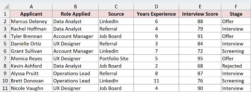
We want Stage first, followed by Applicant and Interview Score.
Here is the formula:
=CHOOSECOLS(A2:F11,6,1,5)
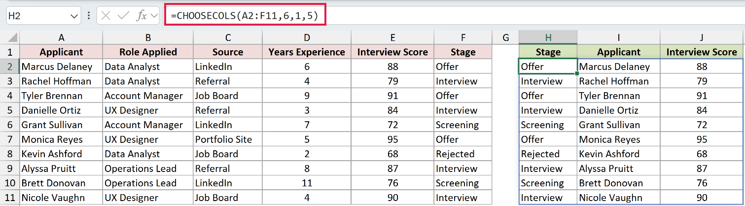
CHOOSECOLS returns column 6 first, column 1 second, and column 5 third. The source table stays in its original order.
Marcus Delaney’s result is Offer, Marcus Delaney, and 88. Monica Reyes’s row returns Offer, Monica Reyes, and 95.
This is handy when a report needs its status or main figure at the left edge.
Example 3: Select Last Columns with Negative Numbers
Now let’s select columns by counting from the right.
Below is the dataset. Columns A through F contain catering event IDs, clients, menu packages, dates, deposits, and balances.
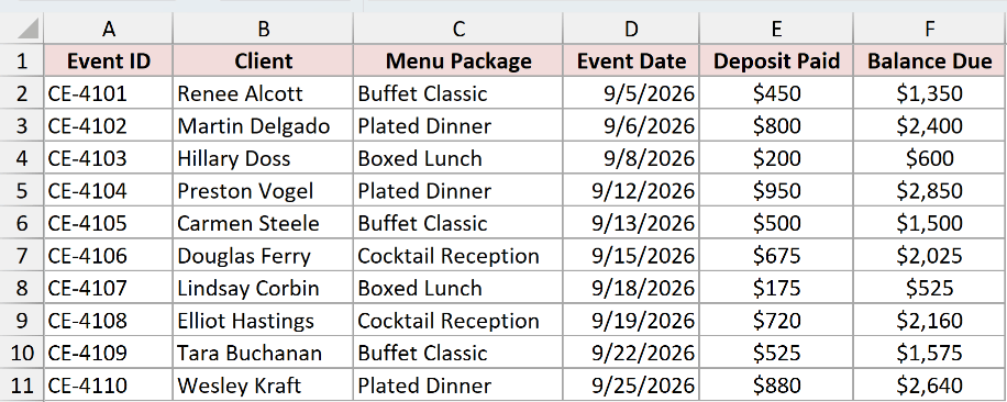
We want the Client column plus the final two money columns.
Here is the formula:
=CHOOSECOLS(A2:F11,2,-2,-1)
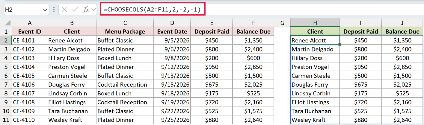
The number 2 returns Client. Then -2 returns Deposit Paid, while -1 returns Balance Due.
Renee Alcott’s row shows $450 and $1,350. Wesley Kraft’s row shows $880 and $2,640.
Negative numbers help when new columns might be inserted in the middle, but the fields you need remain at the right edge.
Example 4: Supply Column Numbers as an Array
This example creates two separate views of the same payroll table.
Below is the dataset. Columns A through F contain eight employees with gross pay, deductions, and net pay.
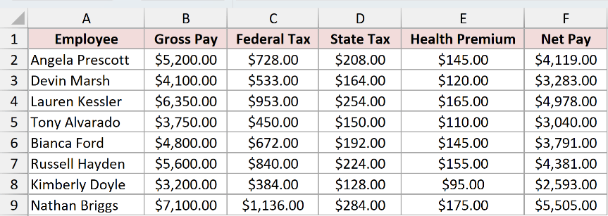
We want a three-column summary view in H2:J9 and a separate three-column tax view directly below it in H12:J19, both using columns H through J.
Here is the formula for the first view:
=CHOOSECOLS(A2:F9,{1,2,6})
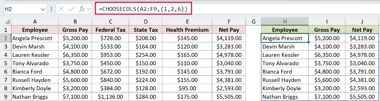
The array constant {1,2,6} returns Employee, Gross Pay, and Net Pay.
Angela Prescott’s row shows $5,200.00 gross pay and $4,119.00 net pay. Nathan Briggs’s row shows $7,100.00 and $5,505.00.
Here is the formula for the second view:
=CHOOSECOLS(A2:F9,HSTACK(1,SEQUENCE(1,2,3)))
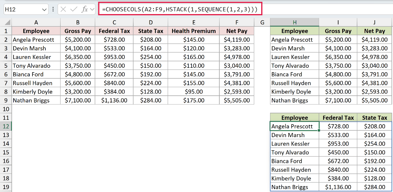
The second view has its own typed header row: Employee, Federal Tax, and State Tax.
SEQUENCE(1,2,3) generates 3 and 4. HSTACK adds 1, producing the column list {1,3,4}.
That list returns Employee, Federal Tax, and State Tax. Angela Prescott’s tax values are $728.00 and $208.00.
The repeated Employee column keeps the second result readable as its own view. This pattern becomes more useful when the source table has dozens of columns.
Example 5: Filter Rows and Select Columns Together
Here’s how to narrow both rows and columns with one formula.
Below is the dataset. Columns A through F contain ten expense reports with employees, categories, submission dates, amounts, and approvers.
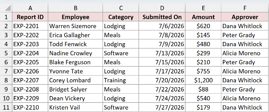
We want only Lodging reports, showing Employee, Submitted On, and Amount.
Here is the formula:
=CHOOSECOLS(FILTER(A2:F11,C2:C11="Lodging"),2,4,5)
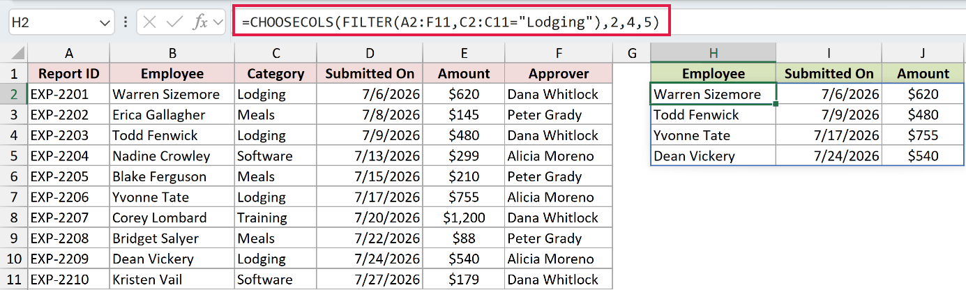
FILTER first keeps the four Lodging rows. CHOOSECOLS then returns columns 2, 4, and 5 from that filtered array.
The spill shows Warren Sizemore on 7/6/2026 for $620 and Todd Fenwick on 7/9/2026 for $480.
It also shows Yvonne Tate on 7/17/2026 for $755 and Dean Vickery on 7/24/2026 for $540.
FILTER alone keeps every source column. Wrapping it with CHOOSECOLS gives you a smaller result without building separate helper columns.
Example 6: Select Columns by Header Name
Finally, let’s avoid hard-coding column positions.
Below is the dataset. Columns A through F contain ten event registrations with attendees, companies, job titles, ticket types, and amounts paid.
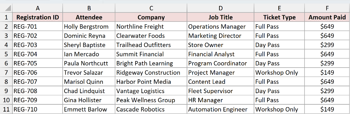
We want CHOOSECOLS to return the fields named in H1:J1.
Here is the formula:
=CHOOSECOLS(A2:F11,XMATCH(H1:J1,A1:F1))
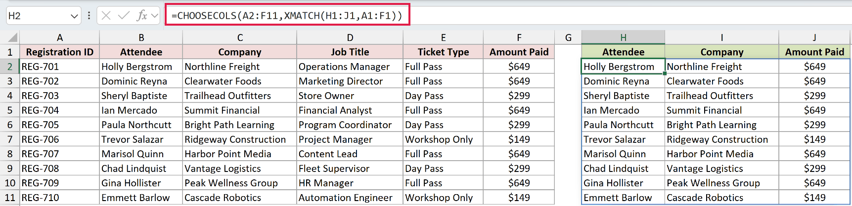
XMATCH turns Attendee, Company, and Amount Paid into the positions 2, 3, and 6. CHOOSECOLS uses those positions to return the fields.
The first row contains Holly Bergstrom, Northline Freight, and $649. The last contains Emmett Barlow, Cascade Robotics, and $149.
You can replace the names in H1:J1 to request different fields without editing the CHOOSECOLS formula.
Pro Tip: XMATCH ignores letter case, but the header wording must otherwise match. A trailing space or renamed header can return #N/A, which then passes into CHOOSECOLS.
Tips & Common Mistakes
- CHOOSECOLS is available in Microsoft 365 and Excel 2024 on Windows and Mac, plus Excel for the web. Excel 2021 and earlier return #NAME?.
- Keep the spill area empty. If another value blocks any destination cell, Excel returns #SPILL!.
- A column number of 0 returns #VALUE!. The same error appears when the absolute number exceeds the array width, such as 7 or -7 for a six-column array.
- CHOOSECOLS returns values, not source formatting. Apply number formats, fills, borders, column widths, and conditional formatting to the spill range separately.
- Include the header row in the array when you want it returned. For example, A1:F11 includes headers, while A2:F11 begins with data.
- You can repeat a column number when the output needs the same field twice.
- Use
=CHOOSECOLS(range,-SEQUENCE(1,COLUMNS(range)))to return every column in reverse order. - CHOOSEROWS follows the same idea for rows. TAKE and DROP work well when adjacent columns sit at an edge of the table.
- Avoid whole-column references such as A:F. Empty rows return as zeros, and the oversized result usually returns #SPILL! instead of spilling.
- The output remains linked to the source. Editing a source value updates the corresponding value in the spilled array.
CHOOSECOLS gives you a clean, live view of selected source columns while leaving the source table alone.
Start with column numbers, then add FILTER, XMATCH, HSTACK, or SEQUENCE when the selection needs to respond to your data.
Related Excel Functions / Articles:
Other Excel articles you may also like:
