
If you want to pull particular rows from a range, the CHOOSEROWS function lets you select them by position.
In this article, I’ll show you how to select, reorder, repeat, and calculate row positions with CHOOSEROWS.
CHOOSEROWS is a dynamic array function. It spills its results across the cells below and beside the formula.
CHOOSEROWS Function Syntax in Excel
The CHOOSEROWS function uses the following syntax:
=CHOOSEROWS(array,row_num1,[row_num2],...)
arrayis the range or array containing the rows you want to return.row_num1is the position of the first row you want to return.[row_num2]is an optional additional row position. You can add more row numbers as needed.
When to Use CHOOSEROWS Function
- Pull specific records from a larger range by their row positions.
- Return the first, last, or every nth row from a dataset.
- Rearrange rows without sorting the source data.
- Repeat a row in the returned array.
- Take the top records after sorting a dataset.
Example 1: Select Specific Rows
Let’s start by selecting several nonadjacent rows.
Below is the dataset of eight inspections, with the site, inspection type, due date, and assigned inspector.

I want to return the first, fourth, and seventh inspections from the range in A2:E9.
Here is the formula:
=CHOOSEROWS(A2:E9,1,4,7)
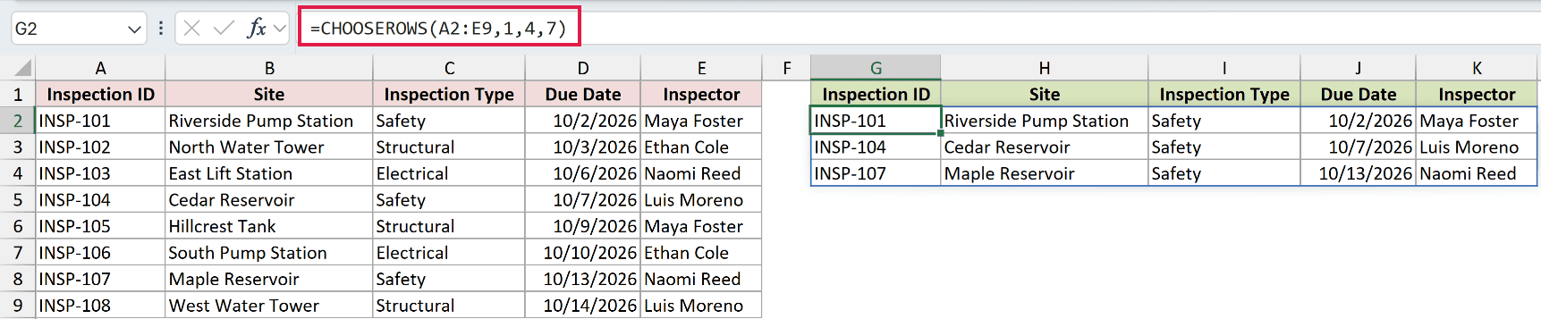
The row numbers are positions within A2:E9, so 1 returns INSP-101, 4 returns INSP-104, and 7 returns INSP-107.
Excel returns all five columns for those three records and spills the result into G2:K4.
Pro Tip: CHOOSEROWS counts positions inside the supplied array. Row 1 here means the first row of A2:E9, not worksheet row 1.
Example 2: Return the Last Three Rows
Negative row numbers make it easy to select from the bottom of a range.
Below is a compost delivery log with the delivery number, garden, quantity, and date received.
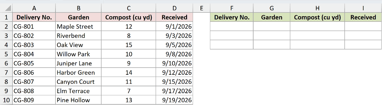
I want to return the final three deliveries from A2:D10 in their original order.
Here is the formula:
=CHOOSEROWS(A2:D10,-3,-2,-1)
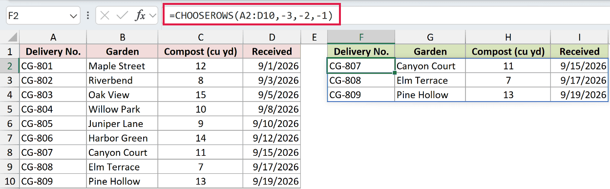
A negative row number counts backward from the end. Here, -1 is the last row, -2 is the second-last, and -3 is the third-last.
Listing them as -3, -2, and -1 returns deliveries CG-807, CG-808, and CG-809 in chronological order.
Pro Tip: If you only need one continuous block from the top or bottom, the TAKE function can be shorter. CHOOSEROWS is more flexible when the positions are not continuous.
Example 3: Rearrange Rows in Excel
CHOOSEROWS can rearrange rows in Excel in any order you specify.
Below is a meeting schedule containing five sessions, their speakers, rooms, and start times.

I want to present the fourth session first, followed by sessions 1, 5, 2, and 3.
Here is the formula:
=CHOOSEROWS(A2:D6,4,1,5,2,3)
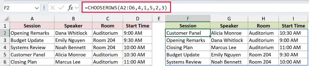
CHOOSEROWS follows the order of the row arguments rather than the order of the source records.
The result begins with Customer Panel, then returns Opening Remarks, Closing Plan, Budget Update, and Systems Review.
The source schedule in A2:D6 stays unchanged.
Example 4: Repeat a Row
You can use the same row number more than once.
Below is a bus route list with each neighborhood, start time, and number of stops.
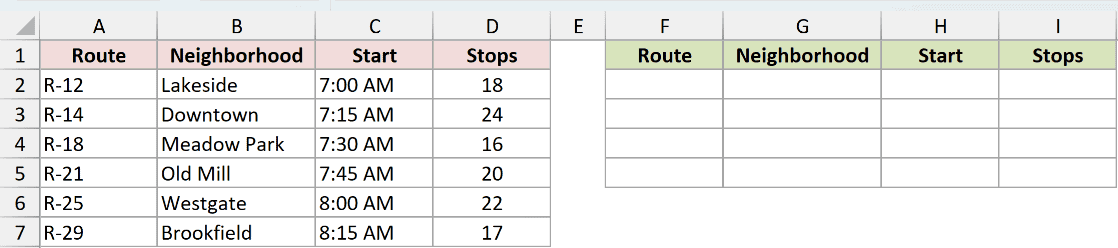
I want to return routes 1, 3, 3, and 6, which repeats the third route in the output.
Here is the formula:
=CHOOSEROWS(A2:D7,1,3,3,6)
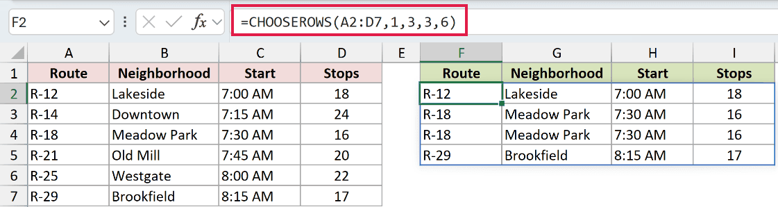
The third position appears twice in the formula, so the R-18 Meadow Park record appears twice in the spilled result.
Excel then returns the sixth position, R-29 Brookfield, as the final row.
Example 5: Return Top Rows After Sorting
CHOOSEROWS becomes more useful when another function first arranges the source array.
Below is a grant review table with the project name, funding request, and review score.
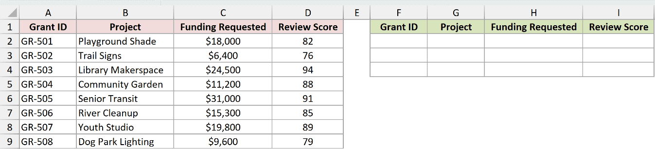
I want to sort the grants by review score and return the three highest-scoring projects.
Here is the formula:
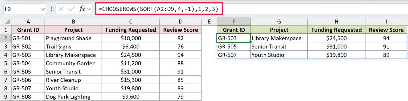
=CHOOSEROWS(SORT(A2:D9,4,-1),1,2,3)
How this formula works:
- The SORT function arranges the records by the fourth column, Review Score, in descending order.
CHOOSEROWS(...,1,2,3)returns the first three rows from that sorted array.- The result contains Library Makerspace, Senior Transit, and Youth Studio, with scores of 94, 91, and 89.
Pro Tip: CHOOSEROWS selects by position. If you need rows that meet a condition, such as every score above 85, use the FILTER function instead.
Example 6: Return Every Other Row
You do not have to type every row position manually.
Below is a list of ten podcast episodes with their topics, lengths, and download counts.
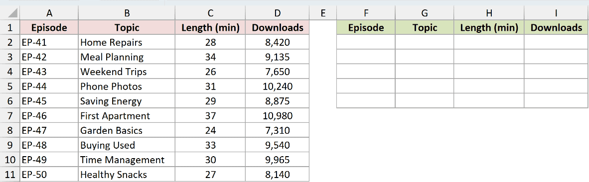
I want to return five alternating records, starting with the first episode in A2:D11.
Here is the formula:
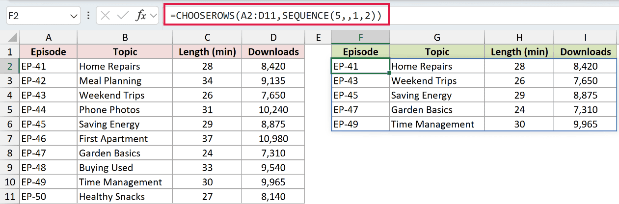
=CHOOSEROWS(A2:D11,SEQUENCE(5,,1,2))
How this formula works:
- The SEQUENCE function creates the row numbers 1, 3, 5, 7, and 9.
- CHOOSEROWS uses those numbers to return EP-41, EP-43, EP-45, EP-47, and EP-49.
- Both functions return dynamic arrays, so the five selected records spill from F2:I6.
Tips & Common Mistakes
- CHOOSEROWS is available in Microsoft 365 and Excel 2024. Earlier perpetual versions, including Excel 2021, do not support it.
- A row number of 0, or one whose absolute value exceeds the number of rows in the array, returns a
#VALUE!error. - Keep the cells in the expected output area empty. Existing content can block the result and cause a
#SPILL!error. - Place the formula outside an Excel Table because spilled array formulas are not supported inside tables.
- The result keeps every column from the source array. Use CHOOSECOLS when you need to select columns instead.
- Use a spilled-range reference such as
F2#when another formula needs the complete CHOOSEROWS result.
I covered how to select rows by position, count from the bottom, reorder and repeat records, and build calculated row lists.
I hope you found this article helpful.
Other Excel articles you may also like:
