How to Move Columns in Excel

If you want to move a column in Excel so it sits somewhere else in your table, you cannot just drag it across and drop it. A plain drag lands the column on top of whatever is already there and wipes it out.

That happens because Excel reads a normal drag as “move these cells here”, not “make room for these cells here”.

But nothing to worry about. There are several reliable ways to slot a column into a new position and push everything else along, and in this article I’ll show you five of them.

Note: This article is about moving one column into a new position, with the other columns shifting over to make room. If you want two columns to exchange places instead, see our guide on how to swap columns in Excel.

Method #1: Use Shift and Drag to Move Columns in Excel

This is the quickest way to move a column when you only need to shift it a position or two. It’s all mouse work, but there’s one key you have to hold at the right moment.

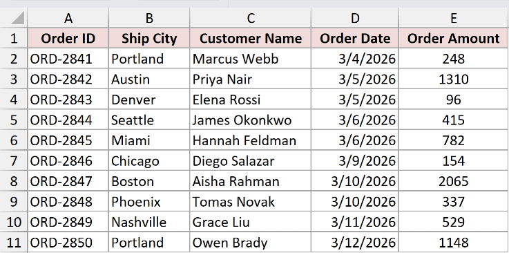
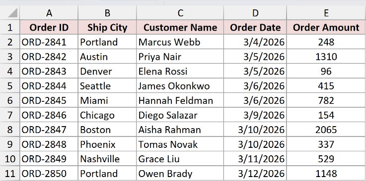
Below I have an order dataset in A1:E11. Ship City sits in column B, wedged between Order ID and Customer Name. I want Customer Name in column B instead, with Ship City pushed over to column C.

Here are the steps to move a column using Shift and drag:

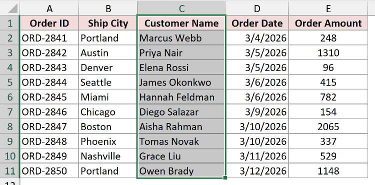
1. Click the column C header to select the entire Customer Name column.

2. Hover over the left border of the selection until the cursor turns into a four-headed move arrow.

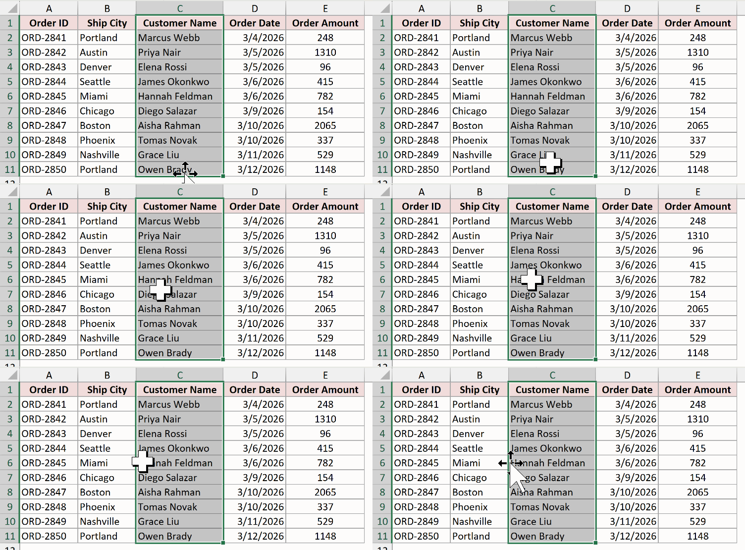
That four-headed arrow is the one you want. If you see a thin black plus sign instead, you’re on the fill handle at the bottom corner of the selection, and dragging that copies your data instead of moving it.

If you never get that arrow and dragging does nothing, the drag-and-drop setting is switched off. Go to File > Options > Advanced and tick “Enable fill handle and cell drag-and-drop”.

3. Hold down the Shift key and drag the column to the left, until the I-beam insertion line sits on the boundary between column A and column B.

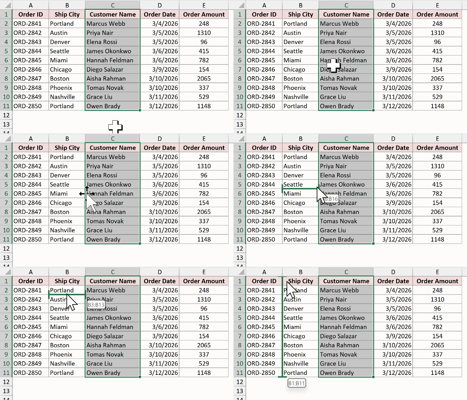
The I-beam is Excel telling you exactly which slot the column will drop into. Ship City and everything to its right slide over to make room.

4. Release the mouse button first, and only then let go of the Shift key.

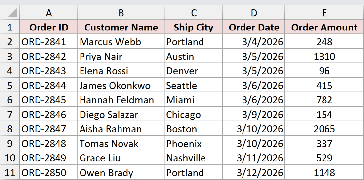
Customer Name is now in column B and Ship City has moved to column C. Nothing was lost along the way.

Note: The order you let go matters. If you release Shift before the mouse button, Excel switches back to a plain move and overwrites the column you dropped onto. Mouse first, Shift second.

Method #2: Apply Cut and Insert Cut Cells to Move Columns in Excel

Here’s another way to do this, and it’s the one I reach for most. Nothing rides on how steadily you hold a key, and the column can jump to the far end of the table just as easily as one position over.

This is the method I’d recommend for most people. It works in every version of Excel, there’s no way to overwrite a column by accident, and a block of adjacent columns moves exactly like a single one.

Below I have the same order dataset in A1:E11. Ship City is in column B and Customer Name is in column C. I want Customer Name moved into column B.

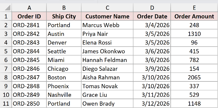
Here are the steps to move a column using Insert Cut Cells:

1. Select any cell in the Customer Name column, such as C2, and press Ctrl + Space to select the whole column.

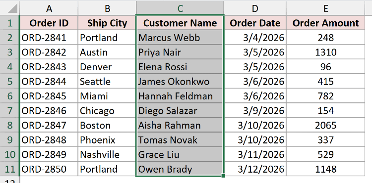
If your data is formatted as an Excel Table, that first press of Ctrl + Space selects only the Table’s portion of the column. Press it again to extend the selection to the full worksheet column.

2. Press Ctrl + X to cut the column. A dashed marching-ants border appears around it.

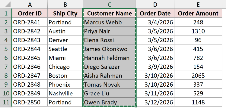
3. Right-click the column B header, the one holding Ship City.

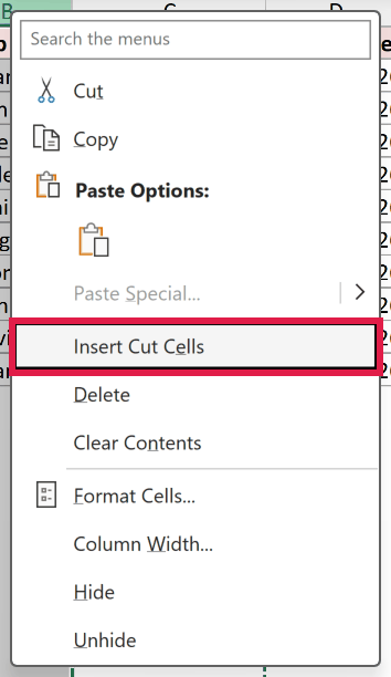
4. Click Insert Cut Cells.

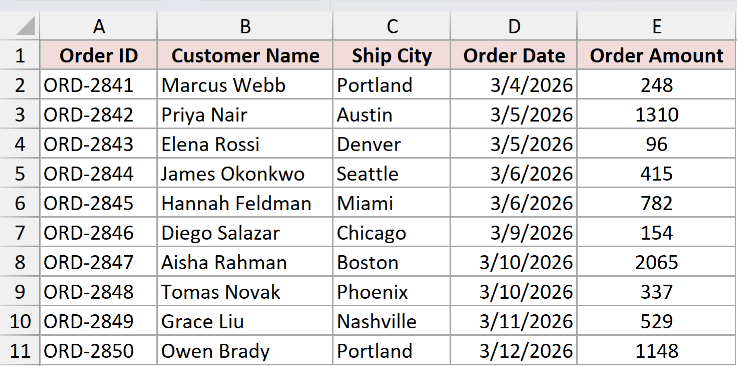
Customer Name drops into column B, and Ship City shifts right into column C. The name says it all: Excel inserts the cut cells rather than pasting over what’s there.

It’s the same cut paste you already use every day. The only difference is that last click, where you tell Excel to make room instead of dropping the cells on top.

Note: Cut only handles one continuous range at a time. If you Ctrl-click two columns that aren’t next to each other and try to cut them, Excel stops you with “That command cannot be used on multiple selections”. Move them one at a time.

Method #3: Use the CHOOSECOLS Function to Move Columns in Excel (Microsoft 365 and Excel 2024)

If you’d rather not touch the original data at all, this one is for you. CHOOSECOLS is a dynamic array function that hands you back the columns you ask for, in the order you ask for them.

CHOOSECOLS does not move your columns. It spills a reordered copy somewhere else on the sheet, and your source table stays exactly as it was.

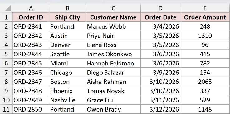
Below I have the same order dataset in A1:E11, with Ship City in column B and Customer Name in column C. I want a copy where Customer Name comes second.

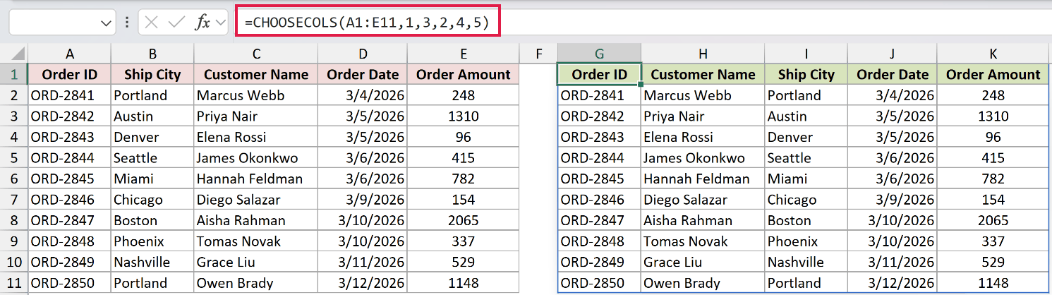
Here is the formula, entered in cell G1:

=CHOOSECOLS(A1:E11,1,3,2,4,5)

How does this formula work?

The first argument, A1:E11, is the whole table including its header row. Everything after that is a column number, and the order you list them in is the order you get back.

So 1, 3, 2, 4, 5 means: give me column 1 (Order ID), then column 3 (Customer Name), then column 2 (Ship City), then columns 4 and 5 as they are.

The result spills across G1:K11 on its own. You write one formula in one cell, and Excel fills the rest of the block.

CHOOSECOLS only exists in Microsoft 365 and Excel 2024. On older versions you’ll get a #NAME? error, so use Method #1 or Method #2 instead.

Note: Every column number has to be a real column in the range. A 0, or a number bigger than the column count, returns a #VALUE! error. Our range is five columns wide, so =CHOOSECOLS(A1:E11,1,3,2,4,6) would fail.

Method #4: Use Power Query to Move Columns in Excel

If you get the same file every month and always have to fix the same column order, this is worth setting up once. Power Query remembers the reorder as a step and re-applies it whenever you refresh.

Below I have the same order dataset in A1:E11. Ship City sits in column B and Customer Name in column C, and I want Customer Name second.

Here are the steps to move a column using Power Query:

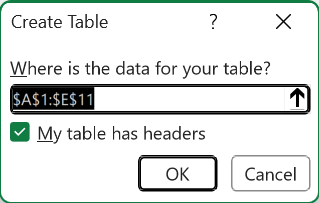
1. Select any cell in the dataset and press Ctrl + T, then click OK to turn it into an Excel Table. Power Query cannot pick up a plain range.

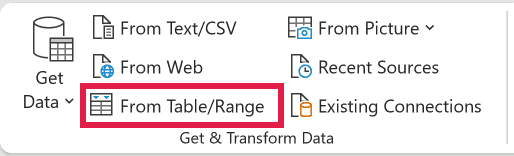
2. On the Data tab, click From Table/Range. The Power Query Editor opens with your data in it.

3. Drag the Customer Name column header to the left, until it sits before Ship City. You can also right-click the header and use Move > Left.

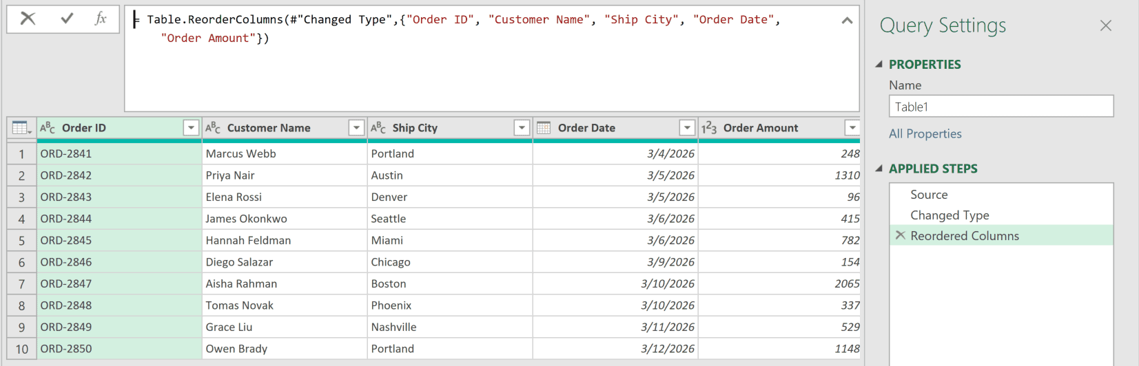
Look at the Applied Steps pane on the right and you’ll see a new step called Reordered Columns. Power Query has written your drag out as M code, using the Table.ReorderColumns function:

= Table.ReorderColumns(#"Changed Type",{"Order ID", "Customer Name", "Ship City", "Order Date", "Order Amount"})

The step spells out the column names, so renaming a column in the source breaks it. Rename first, reorder second, and you’ll avoid that.

4. On the Home tab of the Power Query Editor, click Close & Load.

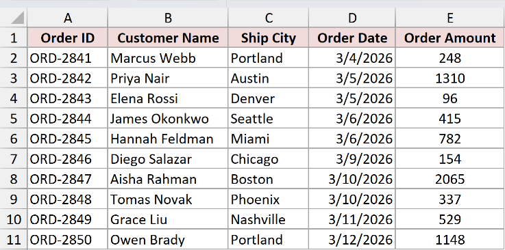
You get a brand new table on a new worksheet, with the columns in the order you wanted. Your original table is untouched.

Note: Power Query does not update itself. When the source data changes, go to Data > Refresh All to pull the new rows through the reorder step.

Method #5: Run a VBA Macro to Move Columns in Excel

If you’re moving the same column on dozens of sheets, or you want this bolted onto a button, a macro does it in one click.

Below I have the same order dataset in A1:E11, with Ship City in column B and Customer Name in column C. The macro moves column C into column B.

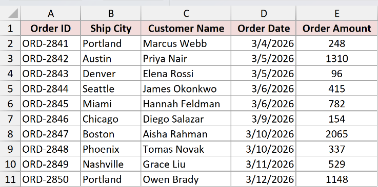
Here is the VBA code:

Sub MoveCustomerNameColumn()
    Columns("C:C").Cut
    Columns("B:B").Insert Shift:=xlToRight
    Application.CutCopyMode = False
End Sub

Sub MoveCustomerNameColumn()
    Columns("C:C").Cut
    Columns("B:B").Insert Shift:=xlToRight
    Application.CutCopyMode = False
End Sub

Ctrl + Z will not undo a macro. Once it runs the change is final, so save your workbook before you try this on real data.

Here are the steps to use this macro:

1. Press Alt + F11 to open the VBA Editor
2. Insert a new module (Insert > Module)
3. Paste the code above
4. Press F5 to run the macro

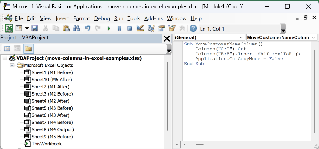
This is Method #2 written out in code. The first line cuts column C.

The second line inserts it at column B and pushes the existing column B to the right, which is exactly what Insert Cut Cells does by hand. The last line clears the clipboard.

To move a different column, change the two letters. Columns("E:E").Cut followed by Columns("C:C").Insert Shift:=xlToRight would move Order Amount into column C.

Note: To keep the macro in the file, save it as a Macro-Enabled Workbook (.xlsm). A normal .xlsx throws the code away when you close it.

Additional Notes About Moving Columns in Excel

• VLOOKUP is the one to watch. Its third argument is a hard-coded number, and it does not update when you move a column. A VLOOKUP counting to column 3 keeps counting to column 3, quietly returning the wrong field. XLOOKUP and INDEX/MATCH point at actual ranges, so they survive a reorder.
• Ordinary formulas are fine. If a formula refers to C2 and you move that cell to B2, Excel rewrites the reference for you.
• Formatting comes along for the ride. Cell formatting, conditional formatting rules, and data validation all travel with the column in Methods #1, #2, and #5.
• Methods #1, #2, #4, and #5 change your data. CHOOSECOLS in Method #3 only shows you a reordered copy, so pick based on whether you actually want the source rearranged.
• Ctrl + Z will undo a drag or an Insert Cut Cells straight away. It will not undo the macro in Method #5.
• Rows work the same way. Select a row instead of a column and both Shift + drag and Insert Cut Cells behave identically, which is covered in our guide on how to rearrange rows in Excel.
• Moving one column is a different job from trading two. If you want Ship City and Customer Name to change places with each other, our article on how to swap columns in Excel covers that.

Frequently Asked Questions

Why does Excel overwrite my data when I drag a column?

Because a drag on its own means “move these cells here”, and Excel does exactly that. Holding Shift while you drag changes it to “insert these cells here”, which pushes the other columns aside instead.

Release the mouse button before you release Shift, or Excel reverts to the overwrite behavior at the last moment.

How do I move multiple columns at once in Excel?

If the columns sit next to each other, select them all and use Method #1 or Method #2 exactly as written. A block of adjacent columns behaves like a single column.

Non-adjacent columns are a different story. Cut refuses to work on a multiple selection, so move them one at a time.

Will moving a column break my formulas?

Cell and range references update themselves, so most formulas keep working. The exception is VLOOKUP, whose col_index_num argument is a plain number that never adjusts.

Move a column inside a VLOOKUP’s table and it silently pulls from the wrong field, with no error to warn you. Check every VLOOKUP after a reorder, or switch to XLOOKUP or INDEX/MATCH.

Why is Insert Cut Cells greyed out in Excel?

Usually because Excel has no cut range waiting. The command only shows up after you press Ctrl + X, so if you pressed Ctrl + C you’ll see Insert Copied Cells there instead, and if you pressed Esc the cut is already cancelled.

The other common cause is a cut that never went through. Excel refuses to cut a non-adjacent multiple selection or a filtered range, which leaves nothing to insert.

Clear the filter, select one unbroken range, then cut. A protected sheet greys the insert commands out too.

How do I move a column inside an Excel Table?

Click the column’s header to select it, then drag it from the edge of the selection to where you want it.

The difference from a normal range is that you can skip the Shift key. A Table always makes room for the column instead of pasting over what’s there, so the insertion line is the only thing you need to watch.

Conclusion

Those are five ways to move a column into a new position and have Excel shift everything else along instead of flattening it.

For everyday work I’d stick with Cut and Insert Cut Cells. It works in every version, and there’s no way to overwrite a column by accident. Whichever one you pick, go check your VLOOKUPs afterwards.

Other Excel articles you may also like:

• How to Shift Cells Down in Excel (8 Easy Ways)
• How to Swap Cells in Excel (3 Easy Ways)
• Insert Column in Excel (Shortcut)
• How to Flip Data in Excel (Columns, Rows, Tables)?