
The DB function in Excel returns an asset’s depreciation for a specified period using the fixed-declining balance method.
It applies a fixed rate to the remaining value, so depreciation is usually higher in earlier periods. An optional month argument handles a partial first year.
In this article, I’ll show you how to build a depreciation schedule, prorate a partial first year, and compare DB with other depreciation methods.
DB Function Syntax in Excel
The DB function needs an asset’s cost, salvage value, useful life, and the period you want to calculate.
=DB(cost, salvage, life, period, [month])
- cost (required) is the asset’s initial cost.
- salvage (required) is the asset’s expected value at the end of its useful life.
- life (required) is the number of periods over which the asset is depreciated.
- period (required) is the period for which you want the depreciation charge. It must use the same units as life.
- month (optional) is the number of months the asset was in service during its first year. Excel assumes 12 when you omit it.
When to Use DB Function
- Calculate depreciation that is highest in the first period and gets smaller over time.
- Build a year-by-year schedule using one fixed declining rate.
- Prorate the first year’s depreciation when an asset enters service partway through the year.
- Compare fixed-declining depreciation with double-declining and straight-line methods.
Example 1: Calculate Depreciation for Two Years
Let’s start with one asset and two annual depreciation charges.
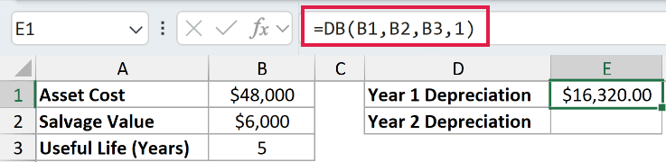
Below is the dataset. The card contains a $48,000 asset cost, a $6,000 salvage value, and a five-year useful life.

We want to calculate the asset’s depreciation for years 1 and 2.
Here is the year 1 formula:
=DB(B1,B2,B3,1)
And here is the year 2 formula:
=DB(B1,B2,B3,2)
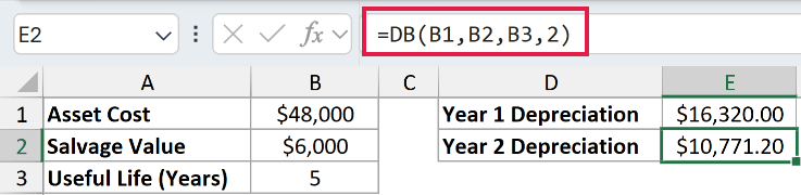
Year 1 returns $16,320.00, while year 2 returns $10,771.20.
Excel derives one fixed rate from the cost, salvage value, and useful life, then rounds that rate to three decimal places.
The first charge applies that rate to the cost. Later charges apply the same rate to a smaller book value, so depreciation falls over time.
Pro Tip: A salvage value of 0 makes the fixed rate equal 1. DB then takes the entire cost in period 1 and returns zero afterward. Use SLN, DDB, or a small token salvage value when that is not the result you need.
Example 2: Spill First-Year Depreciation for Several Assets
Now let’s calculate the first-year charge for a whole equipment fleet.
Below is the dataset. Each row lists an asset, purchase cost, salvage value, and useful life in years.
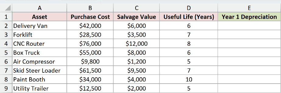
We want one formula to return year 1 depreciation for all eight assets.
Here is the formula:
=DB(B2:B9,C2:C9,D2:D9,1)
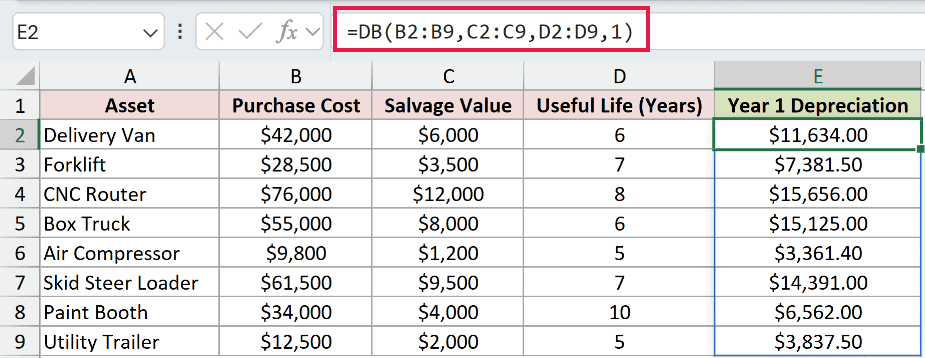
The formula starts in E2 and spills through E9. Each row uses its own cost, salvage value, and useful life.
The result is $11,634.00 for the delivery van and $3,837.50 for the utility trailer.
Pro Tip: Keep E2:E9 empty before entering the formula. Any value in that output range blocks the spill and causes a #SPILL! error.
Example 3: Build a DB Depreciation Schedule
Here’s how to turn the function into a full schedule with a running book value.
Below is the dataset. Column A lists years 1 through 5, and the input table contains a $60,000 cost, $9,000 salvage value, and five-year life.
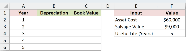
We want annual depreciation in column B and the remaining book value in column C.
Enter this DB formula in B2 and copy it down through B6:
=DB($F$2,$F$3,$F$4,A2)
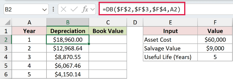
Then enter this book value formula in C2 and copy it down through C6:
=$F$2-SUM($B$2:B2)
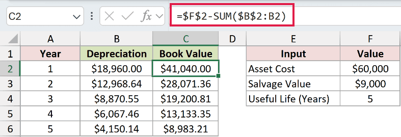
We keep this schedule per-row because Book Value is a running total that depends on the rows above it.
The absolute references keep the three inputs fixed. The period reference changes from A2 through A6 as the DB formula is copied down.
The expanding range in the Book Value formula adds all depreciation through the current year, then subtracts that total from the original cost.
The schedule ends at $8,983.21 against a $9,000 salvage value. DB misses the target slightly because Excel rounds its fixed rate to three decimals.
That small difference is expected. Accountants commonly adjust the final period by hand so the ending book value matches the required salvage value.
Example 4: Prorate a Partial First Year
Next, let’s handle an asset placed in service partway through its first year.
Below is the dataset. It lists six periods beside a $36,000 cost, $4,000 salvage value, five-year life, and nine months in the first year.
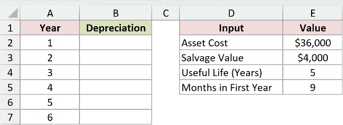
We want one formula to calculate the shortened first year and every later period.
Here is the formula:
=DB(E2,E3,E4,A2:A7,E5)
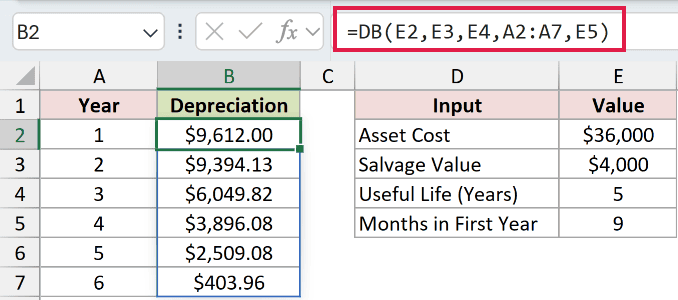
The period range in A2:A7 makes the results spill from B2 through B7.
The month argument means the asset was in service for nine months during its first year. It does not mean the asset was purchased in month nine.
Year 1 returns $9,612.00. The schedule runs for six periods because the final $403.96 charge covers the remaining three months.
VDB is the more flexible option when you need fractional periods or want depreciation to switch to straight-line during the asset’s life.
Example 5: Compare DB, DDB, and SLN
Finally, let’s compare three depreciation methods on the same asset.
Below is the dataset. It lists five years and inputs of $45,000 cost, $6,000 salvage value, and a five-year useful life.

We want to see how each method spreads the $39,000 depreciable amount across five years.
We keep this example per-row because three methods sit side by side for comparison.
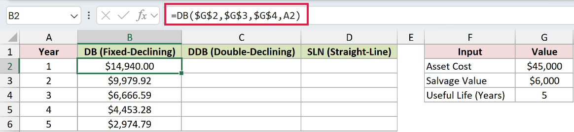
First, enter this DB formula in B2 and copy it down through B6:
=DB($G$2,$G$3,$G$4,A2)
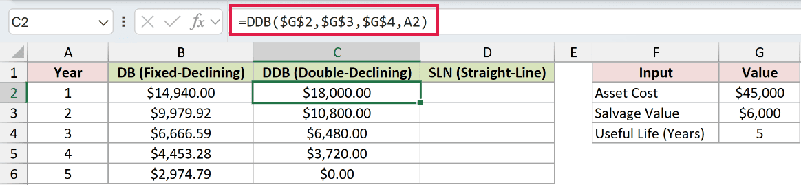
Next, enter this DDB formula in C2 and copy it down through C6:
=DDB($G$2,$G$3,$G$4,A2)
Then enter this SLN formula in D2 and copy it down through D6:
=SLN($G$2,$G$3,$G$4)
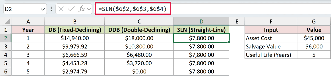
DB starts at $14,940.00 and declines each year. Its five charges total $39,014.58, leaving a book value of $5,985.42.
DDB starts more sharply at $18,000.00, clamps the asset at its $6,000 salvage value in year 4, and returns $0.00 in year 5.
SLN spreads the amount evenly, returning $7,800.00 in every year.
DB has no factor argument. Use DDB when you need 150% or 200% declining balance, and use SLN when you want the same charge every period.
Tips & Common Mistakes
- Keep period and life in the same units. A life entered in years requires periods entered in years too, a convention shared by Excel financial functions such as NPER.
- DB returns #NUM! when period exceeds life without month, or exceeds life plus one when month is used. It also returns #NUM! when month is outside 1 through 12.
- Non-numeric text in any argument returns #VALUE!. Check imported cost, salvage, and life columns for text before troubleshooting the formula.
- In Excel 365, Excel 2024, Excel 2021, and Excel for the web, range inputs spill. Blocked output cells cause #SPILL!, while
@forces one result. - In Excel 2019 and earlier, enter DB for the first row and fill it down. A spill saved in Excel 365 can open as a legacy CSE array in Excel 2019 or 2016 and still calculate every row.
- DB uses one fixed rate based on cost, salvage value, and useful life. DDB supplies a factor, while VDB can switch to straight-line.
- Displayed cents come from cell formatting. Adding the displayed values by hand can differ slightly from a total based on the full stored values.
DB works best when you want one fixed declining rate and a heavier depreciation charge early in an asset’s life.
For partial periods, check the month argument carefully, then compare the completed schedule with the salvage value before using it in your records.
Other Excel articles you may also like:
