
The DELTA function in Excel checks whether two numbers are exactly equal and returns 1 for a match or 0 for a mismatch.
Those numeric flags are useful when checking quantities from two records: you can see which rows match, then add the flags to count them.
The name can be misleading. This function is separate from the Greek delta symbol and doesn’t calculate the difference between two numbers.
It also compares the stored values, so two numbers that look identical after formatting can still return 0.
In this article, I’ll show you how to flag and count matching values, test numbers against zero, and investigate apparently equal numbers that do not match.
DELTA Function Syntax in Excel
The DELTA function takes one required number and an optional second number.
=DELTA(number1, [number2])
- number1 (required) is the first number you want to compare.
- number2 (optional) is the second number. Excel uses zero when you leave it out.
DELTA returns 1 when the numbers are exactly equal and 0 when they aren’t. It never returns the size of the difference.
When to Use DELTA Function
- Flag matching number pairs with 1 and nonmatching pairs with 0.
- Count matching rows by summing a completed DELTA result column.
- Test a column of numbers against zero by leaving out the second argument.
- DELTA is an Engineering function in Excel and follows the familiar Kronecker delta convention used in engineering and math worksheets.
Example 1: Flag and Count Matching Rows
Let’s start with an inventory count check.
Below is the dataset. Column A lists item codes, while columns B and C contain the system and counted quantities.
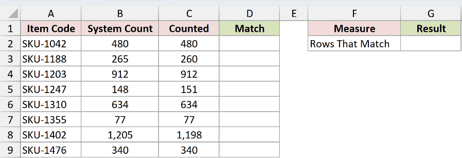
We want to flag every matching row, then count the matches.
Enter this formula in D2 and copy it down through D9:
=DELTA(B2,C2)
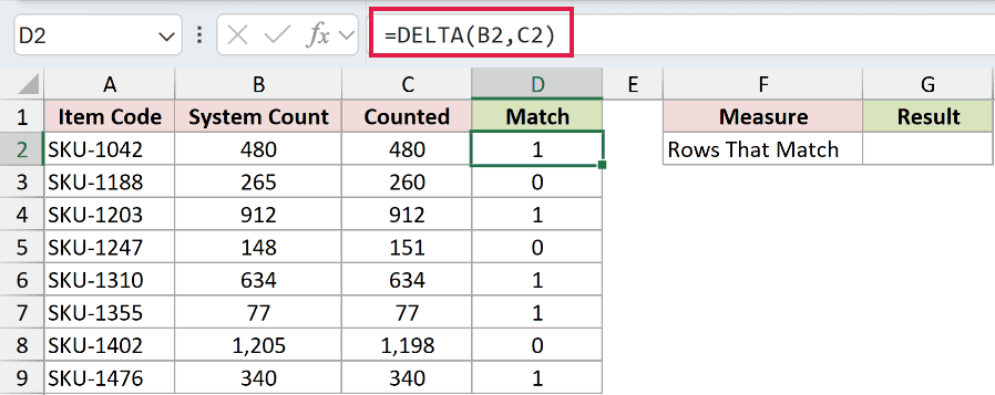
The formula returns 1 when the two counts match and 0 when they don’t.
Now use this formula in G2 to count the 1s:
=SUM(D2:D9)
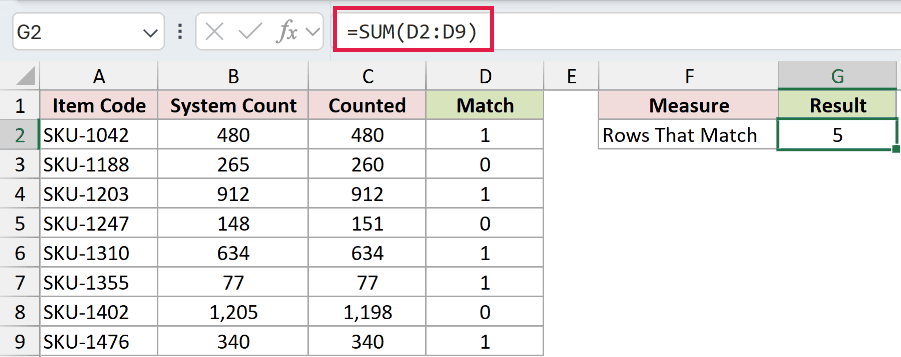
SUM reads the completed Match column and returns 5, so five of the eight inventory rows match.
If you only need the final count, =SUMPRODUCT(--(B2:B9=C2:C9)) compares the ranges without DELTA or a helper column and returns 5.
DELTA earns its place here because the row-level flags stay visible during reconciliation.
Example 2: Test Numbers Against Zero
Here’s a useful shortcut when zero is the value you need to check.
Below is the dataset. Column A lists clearing accounts, and column B contains each closing balance.
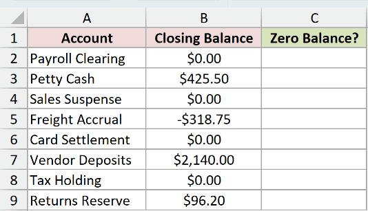
We want to flag every account with a zero balance.
Enter this formula in C2 and copy it down through C9:
=DELTA(B2)
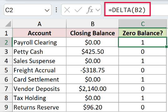
Because the second argument is omitted, Excel compares each balance with zero. The four zero-balance accounts return 1, while every other account returns 0.
COUNTIF is shorter when you only need the total. DELTA is useful when you also want a visible flag beside each account.
Example 3: Numbers Look Equal but Return 0
This next example shows why displayed values can be misleading.
Below is the dataset. It lists cost codes, budgeted and actual amounts, calculated variances, and variance values copied from a report.
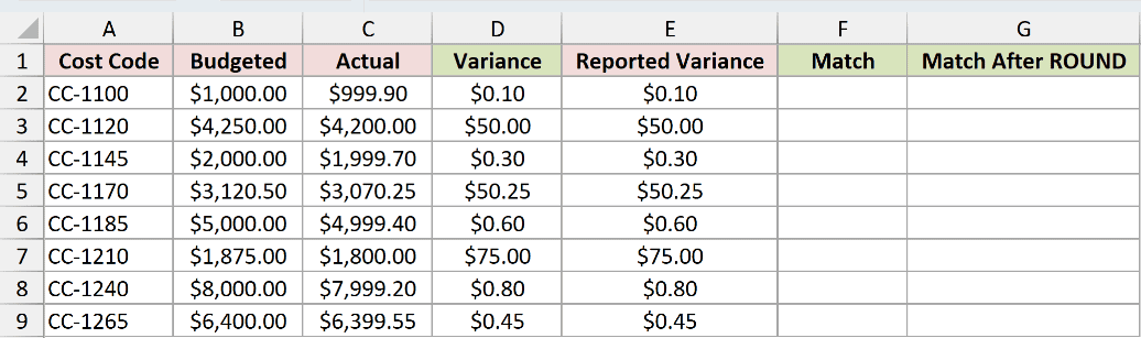
We want to check whether each calculated variance exactly matches its reported value.
First, enter this formula in F2 and copy it down through F9:
=DELTA(D2,E2)
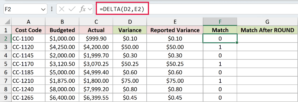
On the first row, D2 and E2 both display $0.10, but DELTA returns 0. Whole-dollar and clean-quarter variances match exactly, while odd-cent variances do not.
Column D subtracts two nearly equal amounts. That subtraction exposes a tiny stored difference below the two displayed decimal places.
Excel compares values at 15 significant digits, so the stored values aren’t equal. A regular equality comparison returns FALSE on the same rows.
This isn’t the familiar 0.1 plus 0.2 story. Excel treats that comparison as equal at its 15-significant-digit precision.
Next, enter this formula in G2 and copy it down through G9:
=DELTA(ROUND(D2,2),ROUND(E2,2))
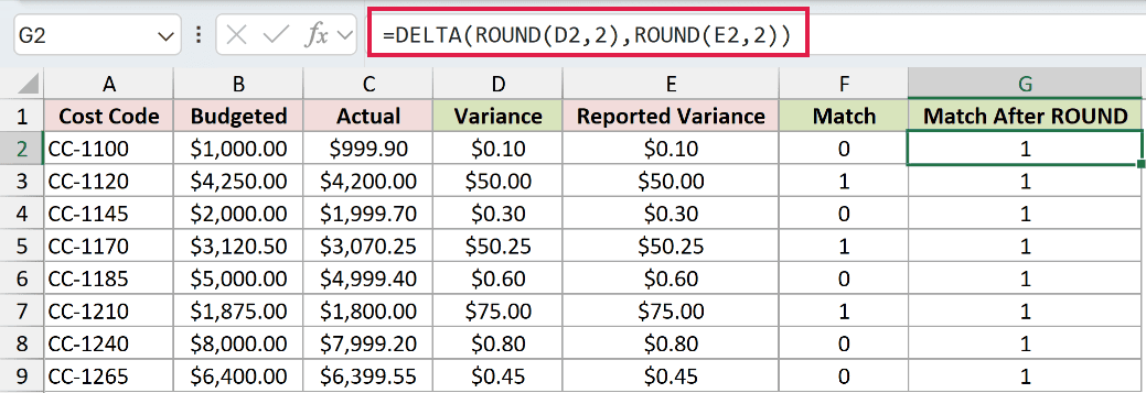
ROUND brings both values to two decimal places before DELTA compares them. All eight rows then return 1.
Pro Tip: Avoid Excel’s Set precision as displayed option as a shortcut. Microsoft warns that it permanently changes stored values, so ROUND is the safer choice.
Example 4: Fix #VALUE! Errors With Text
Finally, let’s compare shipment references that mix numbers and text codes.
Below is the dataset. Column A lists shipments, while columns B and C contain references from the carrier and warehouse exports.
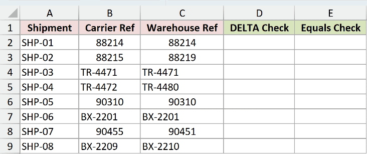
We want a 1 or 0 for every reference pair, regardless of its data type.
Enter this formula in D2 and copy it down through D9:
=DELTA(B2,C2)
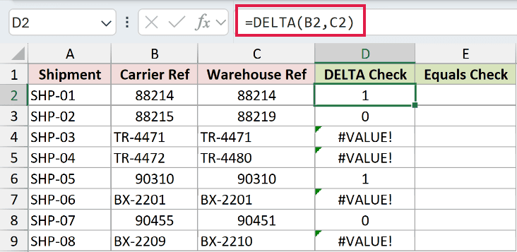
The numeric rows return 1 or 0. Cells D4, D5, D7, and D9 return #VALUE! because those rows contain text references.
Now enter this comparison in E2 and copy it down through E9:
=--(B2=C2)
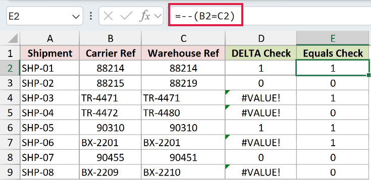
The double unary converts TRUE or FALSE into 1 or 0. It handles both number and text pairs, so all eight rows return usable results.
Text equality is case-insensitive, so bx-2201 and BX-2201 would match. Use EXACT when letter case matters.
For most comparisons, the regular equality test or IF is clearer because both handle numbers, text, and dates.
DELTA fits numeric reconciliation and specialized engineering or math worksheets.
Tips & Common Mistakes
- DELTA accepts numbers, not worksheet ranges. A range argument returns #VALUE!, so enter the first-row formula and copy it down.
- In Microsoft 365, MAP with LAMBDA is the only way to get a spilled column of DELTA results:
=MAP(B2:B9,C2:C9,LAMBDA(x,y,DELTA(x,y))) - DELTA makes an exact comparison and has no tolerance argument. Use ROUND on both values when displayed decimal places define a match.
- Leaving out the second argument tests the first number against zero. This shortcut still returns a numeric 1 or 0.
- DELTA has been built into Excel since Excel 2007. Current versions do not require the Analysis ToolPak.
DELTA is most useful when a numeric check needs 1/0 flags that you can count.
Revisit Example 3 when two numbers look equal and still refuse to match.
Related Excel Functions / Articles:
