
Excel’s PERCENTRANK.INC function returns a value’s relative standing within a numeric dataset as a decimal from 0 through 1, including both endpoints.
It answers a value-to-rank question. PERCENTILE.INC works in the opposite direction by returning the value at a specified percentile.
In this article, I’ll show you how to rank values with PERCENTRANK.INC, estimate ranks for unlisted values, and compare results within separate teams.
PERCENTRANK.INC Function Syntax in Excel
The function uses a reference dataset, a value to rank, and an optional precision setting.
=PERCENTRANK.INC(array, x, [significance])
arrayis the numeric array or range that defines relative standing.xis the value whose percentage rank you want to find.significancesets the number of significant digits returned. It is optional and defaults to three digits.
When to Use PERCENTRANK.INC Function
- Compare each value with all values in a dataset.
- Find the relative standing of a value that is not in the dataset.
- Control the number of significant digits in the calculated rank.
- Rank values within their own teams or categories.
- Include the minimum and maximum values as 0% and 100% endpoints.
Example 1: Rank Every Resolution Time
A full list makes the inclusive endpoints easy to see.
Below is the dataset with request types, resolution times, and relative standing.
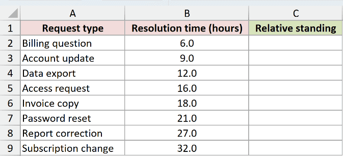
We want to return a percentage rank for every resolution time with one spilling formula.
Here is the formula:
=PERCENTRANK.INC($B$2:$B$9,B2:B9)
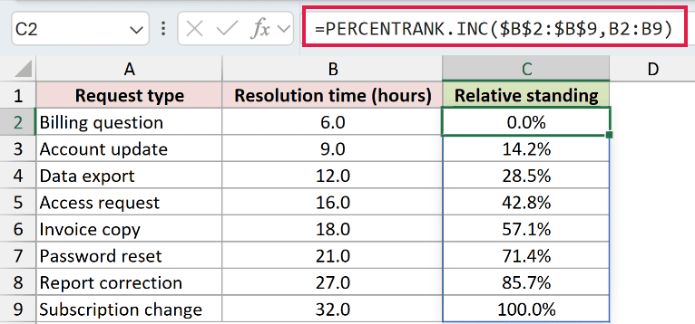
The fixed range $B$2:$B$9 is the comparison dataset. The range B2:B9 supplies all eight values to rank.
Excel returns 0% for 6 hours and 100% for 32 hours. The values between them receive ranks from 14.2% through 85.7%.
In Excel 2021, Excel 2024, and Microsoft 365, the x range spills eight answers from C2. Earlier versions need a per-row formula filled down.
Pro Tip: Format the results as percentages for easier reading. The stored values remain decimals from 0 through 1.
Example 2: Rank an Unlisted Value
The target value does not have to appear in the source list.
Below is the dataset with weekly request volumes, a target of 415 requests, and its percent rank.
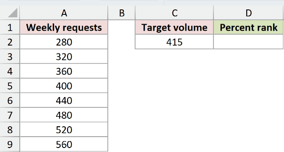
We want to find where 415 falls among the observed weekly volumes.
Here is the formula:
=PERCENTRANK.INC($A$2:$A$9,C2)
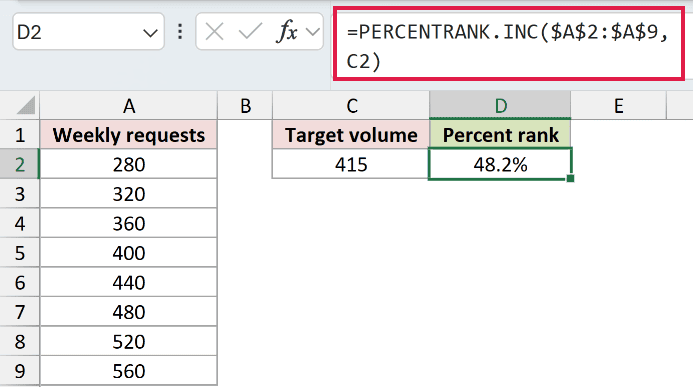
The target sits between 400 and 440. PERCENTRANK.INC interpolates between their ranks and returns 0.482, displayed as 48.2%.
This means 415 is slightly below the midpoint of the observed range’s relative positions.
Pro Tip: An unlisted x value is valid when it falls between the dataset’s minimum and maximum. Excel estimates its position between neighboring values.
Example 3: Set Rank Significance
The optional argument changes the calculated precision.
Below is the dataset with review times, a 15.5-hour target, the default rank, and a one-digit rank.
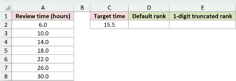
We want to compare the default three-digit result with a result limited to one significant digit.
Here is the default formula:
=PERCENTRANK.INC($A$2:$A$8,C2)
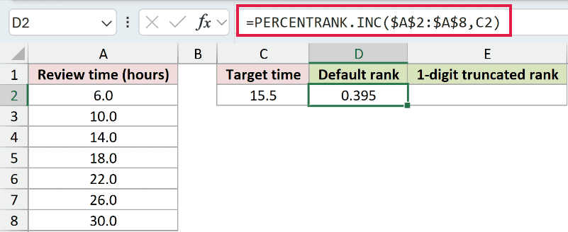
The default setting returns 0.395 for the 15.5-hour target.
Here is the formula with a significance of 1:
=PERCENTRANK.INC($A$2:$A$8,C2,1)
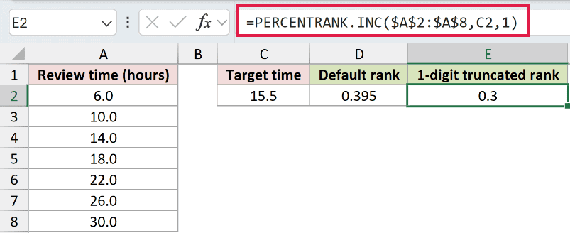
With one significant digit, Excel returns 0.3. It truncates the calculated rank rather than rounding 0.395 up to 0.4.
Pro Tip: Use cell formatting when you only want fewer displayed decimals. The significance argument changes the value returned by the formula.
Example 4: Calculate Rank Within Teams
Sometimes the relevant comparison group is a category, not the entire list.
Below is the dataset with two support teams, task durations, and ranks within each team.
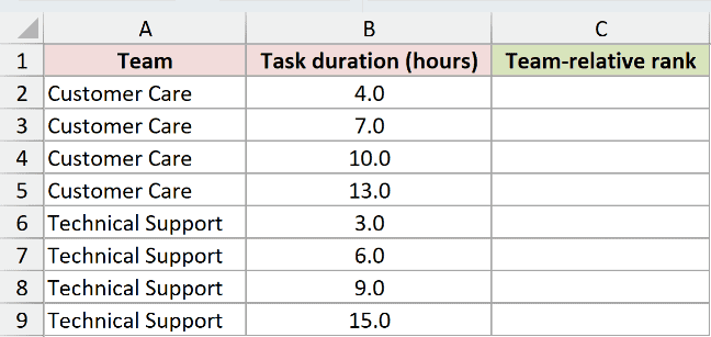
We want to compare each task only with durations from the same team.
Here is the formula in C2:
=PERCENTRANK.INC(FILTER($B$2:$B$9,$A$2:$A$9=A2),B2)
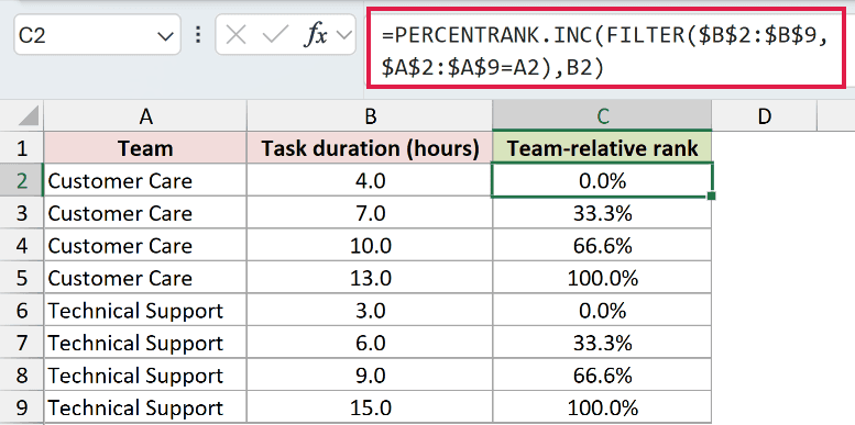
The FILTER function returns the four durations belonging to the team in A2. PERCENTRANK.INC then ranks B2 against that smaller array.
After the formula is filled down, each team’s durations run from 0% to 100% within that team.
Pro Tip: FILTER is available in Excel 2021, Excel 2024, and Microsoft 365. In older versions, use a fixed range for each team’s data.
Example 5: Compare Inclusive and Exclusive Ranks
The endpoint rule determines which percent-rank function to use.
Below is the dataset with benchmark times, the minimum and maximum selected values, and their inclusive and exclusive ranks.
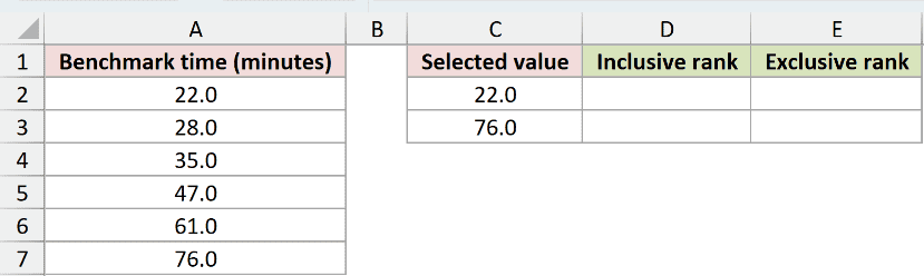
We want to compare how the inclusive and exclusive functions treat the two endpoints.
Here is the inclusive formula in D2:
=PERCENTRANK.INC($A$2:$A$7,C2)
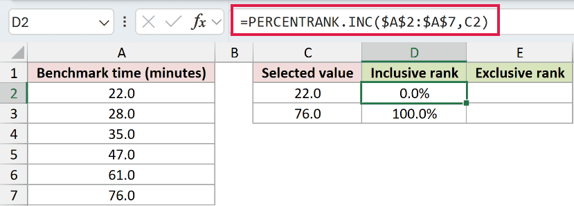
Fill the formula down to D3. PERCENTRANK.INC assigns the minimum value of 22 a rank of 0% and the maximum value of 76 a rank of 100%.
Here is the exclusive formula in E2:
=PERCENTRANK.EXC($A$2:$A$7,C2)
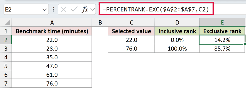
Fill this formula down to E3. PERCENTRANK.EXC excludes 0 and 1 as endpoints.
It returns 14.2% for 22 and 85.7% for 76 in this six-value dataset.
Use the version that matches your statistical definition before interpreting or comparing the ranks.
Tips & Common Mistakes
- PERCENTRANK.INC returns a decimal from 0 through 1. Apply percentage formatting if you want to display 48.2% instead of 0.482.
- The function ranks a known value. PERCENTILE.INC starts with a percentile and returns the corresponding value.
- The optional
significanceargument truncates the result. It does not round it or merely change the cell display. - Keep the
arrayreference fixed when copying a per-row formula. Otherwise, the comparison dataset shifts with each row. - Use PERCENTRANK.EXC when your chosen method excludes the 0% and 100% endpoints.
- An empty array or a
significancevalue below 1 returns a#NUM!error. - The older PERCENTRANK function remains for compatibility. Use PERCENTRANK.INC or PERCENTRANK.EXC in new workbooks.
I covered spilling ranks, interpolation, significance, team-relative comparisons, and the inclusive versus exclusive endpoint choice.
I hope you found this article helpful.
Related Excel Functions / Articles:
