If you want to find the value below which a given percentage of your data falls, the PERCENTILE function gives it to you in one step.
You hand it your numbers and a percentile like 0.9, and it returns the cutoff for that point.
PERCENTILE returns a single value. But if you feed its k argument a range of percentiles, it spills one result per k into the cells below.
PERCENTILE Function Syntax in Excel
Here is the syntax for the PERCENTILE function.
=PERCENTILE(array, k)
- array (required) – the range of numbers (your data set).
- k (required) – the percentile you want, as a number from 0 to 1 (0.9 = the 90th percentile). k can also be a range or array, in which case PERCENTILE spills one result per k.
When to Use PERCENTILE Function
Here are some everyday situations where PERCENTILE comes in handy.
- Setting test or score cutoffs, like the mark you need to land in the top 10%.
- Building salary bands by splitting pay into percentile ranges.
- Tracking response-time or latency SLAs, where teams report the 95th percentile instead of the average.
- Trimming outliers by cutting off the top and bottom few percent of values.
- Sorting people or products into performance tiers and deciles.
Example 1: Find the 90th percentile
Let’s start with a simple grading example.
Below is the dataset with student scores in column A (A2:A13). We want to drop the 90th percentile into cell C2.
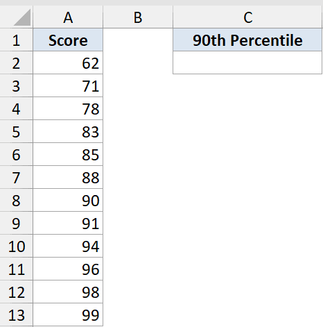
We want the score that 90% of students fall at or below.
Here is the formula:
=PERCENTILE(A2:A13,0.9)
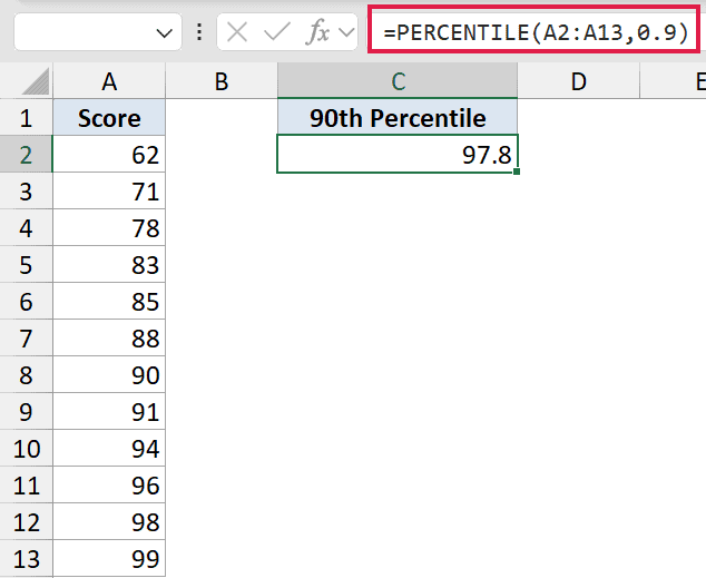
How this formula works: k is 0.9 for the 90th percentile. The result, 97.8, is the cutoff, so 90% of the scores sit at or below it.
Because Excel interpolates between ranked values, 97.8 is not necessarily a score anyone actually got.
Pro Tip: k goes from 0 to 1, not 0 to 100. Type 0.9 or 90%, never 90. Anything above 1 returns a #NUM! error.
Example 2: Get quartiles with PERCENTILE
Quartiles are just percentiles at the quarter marks, so PERCENTILE handles them easily.
Below is the dataset with salaries in column A (A2:A13). To the right, column C lists the quartiles and column D holds each value.
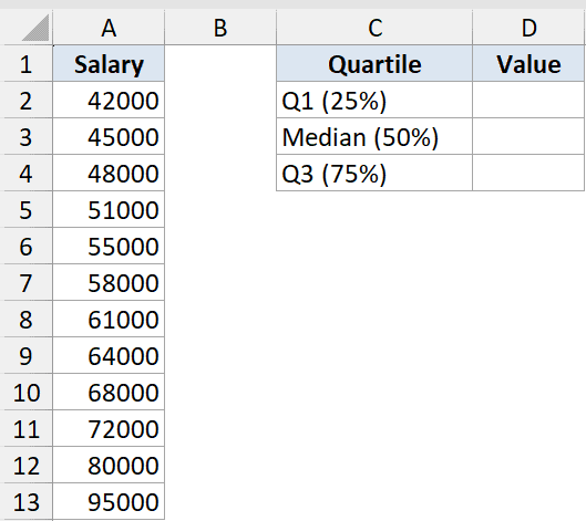
We want the 25th, 50th, and 75th percentiles (the three quartiles) of the salaries.
Here is the formula:
=PERCENTILE(A2:A13,0.25)
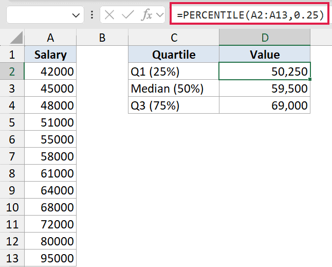
This returns 50,250 for Q1. You get the other two with =PERCENTILE(A2:A13,0.5) (59,500) and =PERCENTILE(A2:A13,0.75) (69,000).
How this formula works:
- 0.25, 0.5, and 0.75 give you Q1, the median, and Q3.
- The median (0.5) is the middle salary, splitting the group in half.
- PERCENTILE lets you pick any cut point, not just quarters.
Quick modern note: =QUARTILE(A2:A13,1) returns the same Q1. QUARTILE is just PERCENTILE locked to quarter points.
Example 3: All percentiles in one formula
Now for the dynamic-array way. Instead of writing five separate formulas, you can compute several percentiles at once.
Below is the dataset reusing the same salaries in A2:A13. Column C holds five k values (0.1, 0.25, 0.5, 0.75, 0.9) in C2:C6, and column D will hold the spilled results.
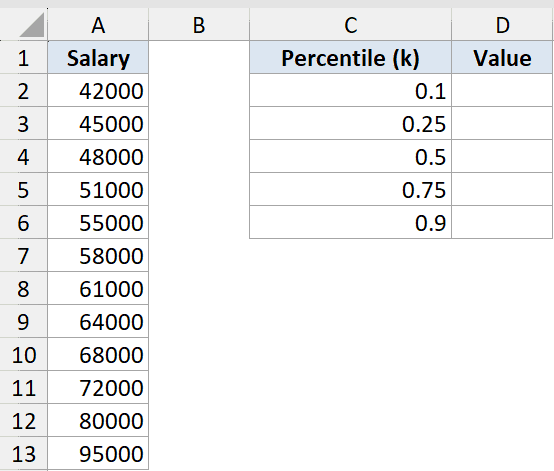
We want five percentiles (10th, 25th, 50th, 75th, 90th) computed at once instead of writing five formulas.
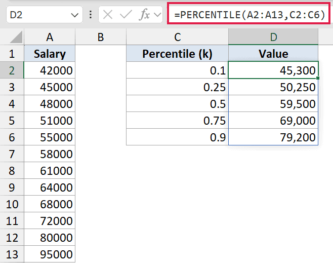
Here is the formula:
=PERCENTILE(A2:A13,C2:C6)
How this formula works:
- Pointing k at the range C2:C6 makes PERCENTILE return one result per k.
- The answers spill down D2:D6 automatically (45,300 / 50,250 / 59,500 / 69,000 / 75,800).
- Edit any k value and the matching result updates on its own.
- This needs Excel 365 or 2021 for the spill to work.
Pro Tip: You can also type the k values straight into the formula as an array constant, e.g. =PERCENTILE(A2:A13,{0.1;0.25;0.5;0.75;0.9}). Semicolons spill down a column, commas spill across a row.
Example 4: PERCENTILE.INC vs PERCENTILE.EXC
Excel has two newer twins for this function, and they don’t always agree.
Below is the dataset with eight numbers in column A (A2:A9). Column C lists the two function names and column D holds the 20th percentile from each.
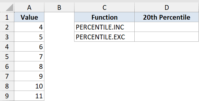
We want to see how the inclusive and exclusive versions differ on the same data at k=0.2.
Here is the formula:
=PERCENTILE.INC(A2:A9,0.2)
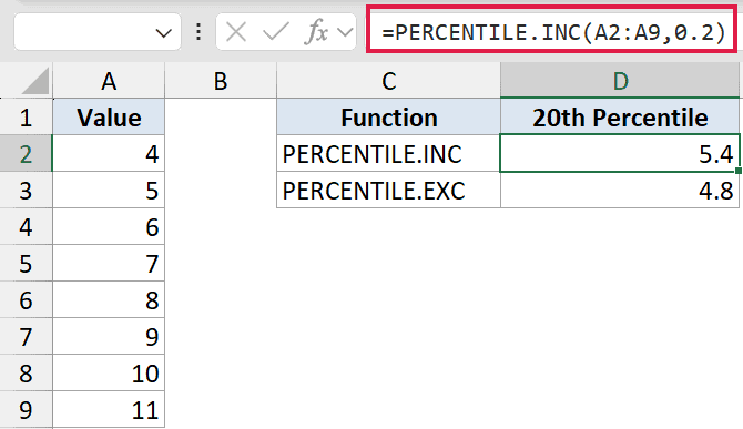
This returns 5.4. The companion =PERCENTILE.EXC(A2:A9,0.2) returns 4.8 on the same data.
How this formula works:
- PERCENTILE.INC is identical to PERCENTILE: inclusive, k from 0 to 1, endpoints allowed.
- PERCENTILE.EXC is exclusive, with k strictly between 0 and 1, and it pushes percentiles slightly outward.
- That is why INC gives 5.4 and EXC gives 4.8 here.
Pro Tip: PERCENTILE.EXC only accepts k between 1/(n+1) and n/(n+1). With 8 values that is roughly 0.11 to 0.89, so very low or very high percentiles return #NUM!.
Example 5: Set a 95th-percentile cutoff and flag rows
Here is the classic SLA pattern, where one slow outlier matters more than the average.
Below is the dataset with page load times in column A (A2:A13). Column B holds a status flag for each row, and the 95th-percentile cutoff lives in D2.
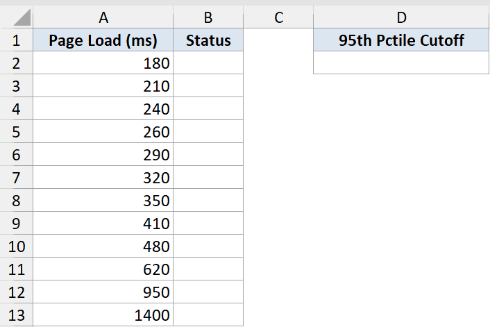
We want the 95th-percentile load time as a threshold, then flag any row at or above it.
Here is the formula:
=PERCENTILE(A2:A13,0.95)
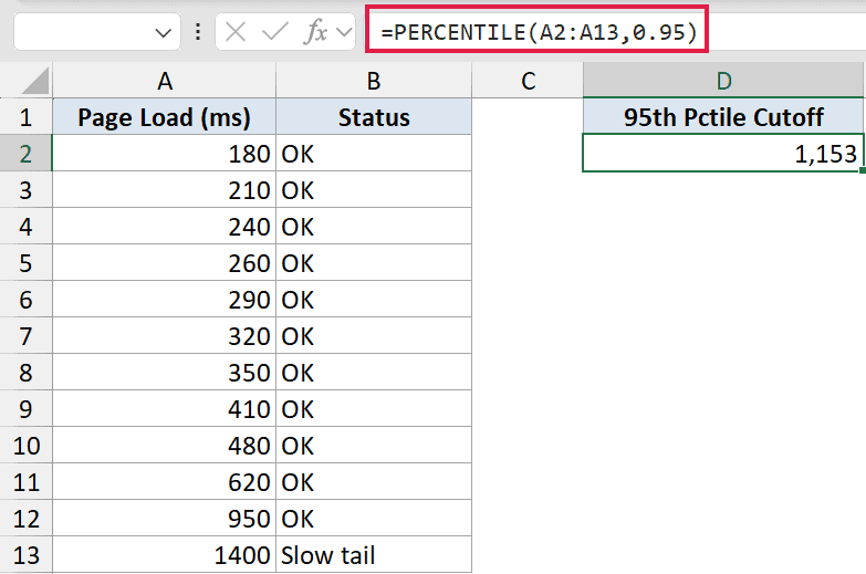
This returns a cutoff of 1,152.5 in D2. The flag column B then uses =IF(A2>=$D$2,"Slow tail","OK") filled down B2:B13, and only the 1,400 ms row flags “Slow tail”.
How this formula works:
- PERCENTILE finds the cutoff, about 1,153 ms.
- The IF column compares each load time to the locked $D$2 cutoff.
- Only the 1,400 ms outlier lands in the slow tail.
- This is the SLA pattern: report the 95th percentile instead of the average so one slow outlier does not get averaged away.
Tips & Common Mistakes
- k is 0 to 1, not 0 to 100 (the most common error). Anything above 1 or below 0 returns #NUM!.
- PERCENTILE = PERCENTILE.INC. Use PERCENTILE.EXC only when you need the exclusive definition, and remember it rejects very high or very low k values.
- The result is usually interpolated, so it may be a number that does not appear in your data. That is expected.
- Text and blank cells are ignored, which changes the count and shifts every percentile.
- PERCENTILE is legacy. For new work use PERCENTILE.INC (identical results), since it is the future-proof name.
That is everything you need to start pulling percentiles out of any data set.
Start with plain PERCENTILE for cutoffs and quartiles, then reach for the spill trick when you want several percentiles at once.
Related Excel Functions / Articles: