
The RANK.AVG function in Excel returns a number’s rank within a list, assigning the average of the occupied positions when values tie.
You can rank from largest to smallest or reverse the order for measures such as completion time. The tie rule is what distinguishes RANK.AVG from RANK.EQ.
In this article, I’ll show you how to rank values in either direction, handle tied scores, and rank entries within a group.
RANK.AVG Function Syntax in Excel
RANK.AVG compares a number with a reference list and averages the positions occupied by any ties.
=RANK.AVG(number, ref, [order])
- number (required) is the number you want to rank. Use a single cell, or a range for multiple results in Excel 2021, Excel 2024, and Microsoft 365.
- ref (required) is the reference list of numbers you’re ranking against. Lock this range with dollar signs when copying formulas down.
- order (optional) controls the direction. Use
0, or omit it, for largest first. Use1for smallest first. Any nonzero value means ascending order.
RANK.AVG averages the rank positions, not the underlying scores. You’ll see exactly what that means in the first example.
When to Use RANK.AVG Function
- Assign league positions when teams with equal points should share the average of their occupied places.
- Rank golf scores from lowest to highest while accounting for ties.
- Compare branch performance when your reporting rules call for averaged ranks.
- Add a complete column of ranks with one formula in Excel 2021, Excel 2024, and Microsoft 365.
- Rank employees against others in the same group by using a separate reference range for each group.
Example 1: Rank League Points From Highest to Lowest
Let’s start with a league table where two pairs of teams have equal points.
Below is the dataset. Column A lists the teams, and column B contains their points in rows 2 through 9.
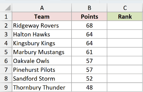
We want the highest points total to rank first, with tied teams sharing an average position.
Here is the formula to enter in C2 and copy down through C9:
=RANK.AVG(B2,$B$2:$B$9,0)
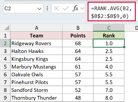
B2 supplies the team’s points. The locked range $B$2:$B$9 keeps all eight teams in the comparison, and 0 puts the largest total first.
Ridgeway Rovers has 68 points, so C2 displays 1.0. Halton Hawks and Kingsbury Kings both have 64 points, and each receives 2.5.
Those two teams occupy second and third place. RANK.AVG gives both the average of those positions.
Marbury Mustangs receives 4.0 because three teams have more points.
Oakvale Owls and Pinehurst Pilots both have 57 points. They occupy fifth and sixth place, so each receives 5.5.
We’re using separate row formulas here so you can follow the locked comparison range. Example 4 shows how to return every rank with one formula.
Pro Tip: Format the Rank column with one decimal place, as shown here. Whole-number formatting can hide a rank such as 2.5, making the tie rule harder to see.
Example 2: Rank Golf Scores From Lowest to Highest
Now let’s reverse the direction, because a lower golf score is better.
Below is the dataset. Column A contains eight player names, and column B lists their round scores, including two players on 71 and three on 75.
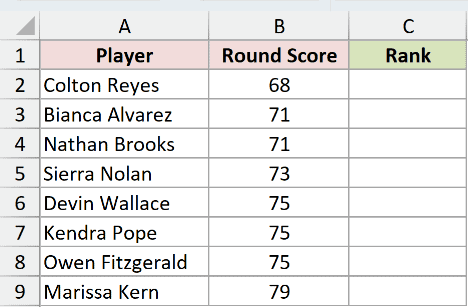
We want the lowest score to rank first while keeping the same average-rank rule for ties.
Here is the formula to enter in C2 and copy down through C9:
=RANK.AVG(B2,$B$2:$B$9,1)
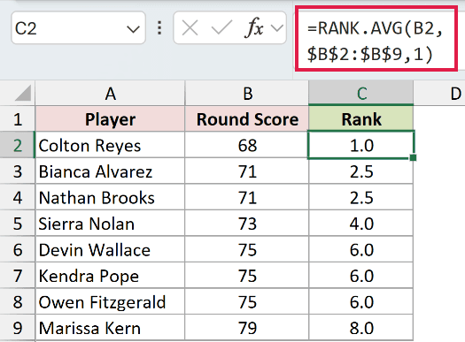
The final argument is now 1. That switches to ascending order, so Colton Reyes’s score of 68 earns 1.0.
Bianca Alvarez and Nathan Brooks both score 71. Their shared rank is 2.5, because they occupy second and third place.
The three players on 75 occupy fifth, sixth, and seventh place. Their average rank displays as 6.0 for Devin Wallace, Kendra Pope, and Owen Fitzgerald.
A tied rank doesn’t have to have a fractional part. A whole-number result can still be an average of several occupied positions.
This example stays per-row to make the change in order easy to compare with Example 1. The spilling approach comes in Example 4.
Example 3: RANK.EQ vs RANK.AVG for Tied Scores
Here’s the difference that matters when choosing between these two functions.
Below is the dataset. Column A lists eight branches, and column B holds service scores, with two branches scoring 92 and three scoring 88.
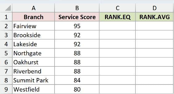
We want to compare shared top ranks with averaged ranks for exactly the same scores.
Here is the RANK.EQ formula to enter in C2 and copy down through C9:
=RANK.EQ(B2,$B$2:$B$9,0)
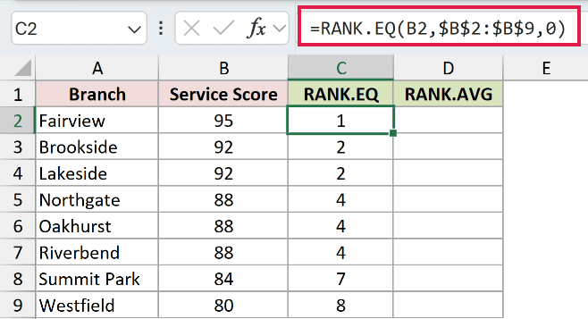
RANK.EQ gives both branches on 92 a rank of 2. It gives all three branches on 88 a rank of 4.
No branch ranks 3, 5, or 6 because RANK.EQ skips the positions used by ties. RANK.AVG averages those occupied positions, giving 2.5 and 5.0.
And here is the RANK.AVG formula to enter in D2 and copy down through D9:
=RANK.AVG(B2,$B$2:$B$9,0)
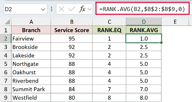
RANK.AVG gives Brookside and Lakeside 2.5 each. Northgate, Oakhurst, and Riverbend receive 5.0 each, averaging fourth, fifth, and sixth place.
Both methods leave the next branch, Summit Park, in seventh place. Column C displays 7, while column D displays 7.0 because it uses one decimal place.
The decimal formatting makes the comparison readable, but it doesn’t create the difference. The functions apply different rules to tied scores.
Pro Tip: Choose RANK.EQ when tied entries should share their highest position, and RANK.AVG when they should share the average position. They’re sibling functions introduced in Excel 2010, so choose by tie policy, not age.
Example 4: Rank a Column With One Formula
Let’s return all eight ranks without copying a formula down.
Below is the dataset. Column A lists warehouses, and column B contains their orders shipped in B2:B9.
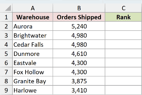
We want one formula to rank every warehouse from most orders shipped to fewest.
Here is the formula to enter once in C2:
=RANK.AVG(B2:B9,B2:B9,0)
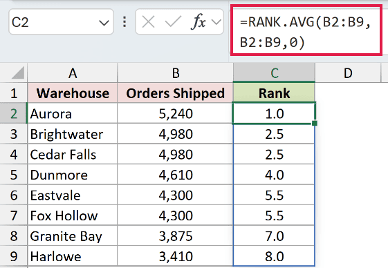
In Excel 2021, Excel 2024, and Microsoft 365, the results spill into C2:C9. You don’t fill down this formula.
The first B2:B9 supplies all eight numbers to rank. The second B2:B9 supplies the comparison list used for each number.
Aurora’s 5,240 orders earn 1.0. Brightwater and Cedar Falls each shipped 4,980 orders, so both receive 2.5.
Eastvale and Fox Hollow each shipped 4,300 orders and receive 5.5. The spill displays 1.0, 2.5, 2.5, 4.0, 5.5, 5.5, 7.0, 8.0.
Neither reference needs dollar signs here because we’re entering one formula once. The earlier examples lock the comparison range because those formulas are copied.
Ranking and sorting do different jobs. RANK.AVG adds a position without moving any rows. SORT or SORTBY reorders the data and doesn’t add a rank number.
Pro Tip: Keep C3:C9 empty before entering the formula in C2. An occupied cell in that output range can cause #SPILL!. Edit the formula in C2 to change the whole spilled result.
Example 5: Rank Technicians Within Each Service Center
Finally, let’s give each service center its own ranking.
Below is the dataset. Columns A through C contain technician names, service centers, and jobs completed. Midtown occupies rows 2 through 6, and Riverside rows 7 through 11.
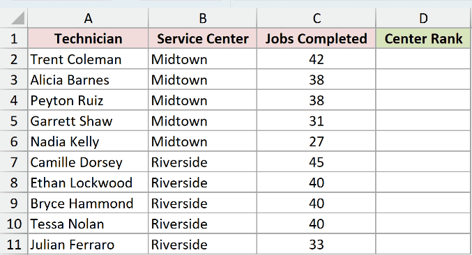
We want to rank each technician against colleagues at the same center, with the most completed jobs first.
Here is the Midtown formula to enter in D2 and copy down through D6:
=RANK.AVG(C2,$C$2:$C$6,0)
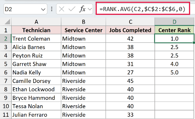
The reference range $C$2:$C$6 includes only Midtown’s job counts. Trent Coleman’s 42 jobs earn 1.0, while Alicia Barnes and Peyton Ruiz each receive 2.5 for 38 jobs.
For Riverside, enter this formula in D7 and copy it down through D11:
=RANK.AVG(C7,$C$7:$C$11,0)
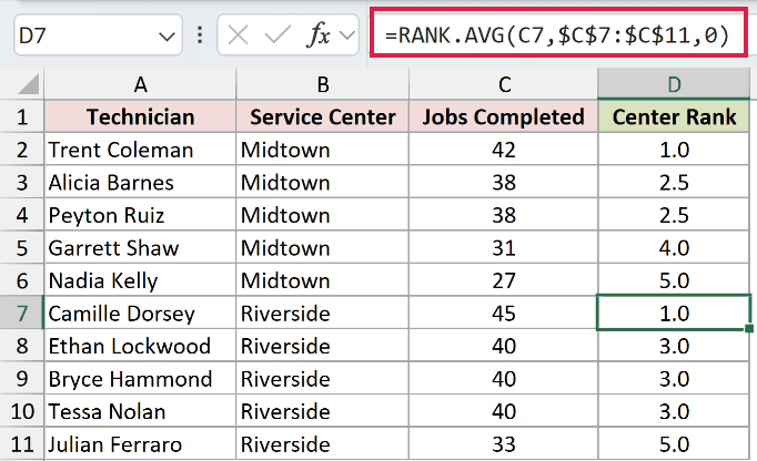
This time, $C$7:$C$11 contains only Riverside’s counts. Camille Dorsey earns 1.0 for 45 jobs.
Ethan Lockwood, Bryce Hammond, and Tessa Nolan each completed 40 jobs. They occupy second through fourth place within Riverside, so each receives 3.0.
These are separate copied-down formulas because each group needs its own fixed comparison range. Copying the Midtown formula into Riverside would retain the wrong group.
The service-center names don’t act as criteria. The group boundaries come entirely from the ranges you supply, so keep each center’s records together for this setup.
Pro Tip: Check both group ranges whenever you add or move technicians. This setup ranks the rows inside $C$2:$C$6 and $C$7:$C$11; it doesn’t automatically select people by the center name in column B.
Tips & Common Mistakes
- Check the direction first. An omitted
orderor0means largest first. Use1when smaller values should receive the best ranks. - Keep numbers numeric. RANK.AVG ignores text, logical values, and blanks in
ref. Numbers stored as text are skipped, so they aren’t counted in the ranking. - Check a missing-number error. If the number you’re ranking isn’t present in
ref, RANK.AVG returns#N/A. Confirm that the comparison range includes the intended value. - Match the formula to your Excel version. RANK.AVG has been available since Excel 2010. Copied-down single-cell formulas work in every version with the function, including older releases. Only Example 4’s automatic spill requires Excel 2021, Excel 2024, or Microsoft 365.
- Watch for implicit intersection. Excel adds
@to preserve legacy behavior in workbooks from older versions. An@before a range argument returns one result instead of the spilled column. For Example 4, delete the@so your formula matches the one shown. - Don’t substitute legacy RANK for averaged ties. RANK remains available for backward compatibility and handles ties like RANK.EQ. No modern Excel function replaces RANK.AVG’s tie-averaging behavior.
- Choose the output you need. LARGE and SMALL return the value at a chosen position. PERCENTRANK.INC expresses relative standing as a proportion. Those are different outputs from RANK.AVG’s position number.
I covered ranking in both directions with order and how RANK.AVG averages the positions occupied by tied values.
I also showed the RANK.EQ comparison, a full column of ranks from one formula, and separate rankings for each group.
Other Excel articles you may also like:
