
The T.DIST.2T function in Excel returns the two-tailed probability for a Student’s t statistic and specified degrees of freedom.
That probability is commonly used as a p-value. It tells you how unusual the observed t statistic would be if the null hypothesis were true.
In this article, I’ll show you how to calculate p-values from t statistics, handle a negative t statistic, and work from summary statistics.
T.DIST.2T Function Syntax in Excel
The function requires a t statistic and the degrees of freedom for the test.
=T.DIST.2T(x,deg_freedom)
- x (required) is the nonnegative t statistic for which you want the two-tailed probability.
- deg_freedom (required) is the number of degrees of freedom.
When to Use T.DIST.2T Function
- Convert one or more calculated t statistics into two-tailed p-values.
- Run a one-sample t-test, which Excel’s T.TEST function cannot do, by calculating the t statistic and passing it to T.DIST.2T.
- Recreate the p-value column for regression coefficients from their coefficients and standard errors.
- Calculate a two-sample p-value when you have summary statistics but not the underlying observations.
Example 1: Convert t Statistics to p-Values
Let’s start with a results log from six retail pilot programs.
Below is the dataset. Columns B and C hold each t statistic and degrees of freedom, while column D will hold the p-values.
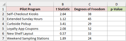
We want one formula to convert all six pairs of inputs into two-tailed p-values.
Here is the formula:
=T.DIST.2T(B2:B7,C2:C7)
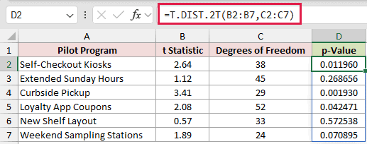
The two aligned ranges let T.DIST.2T use the t statistic and degrees of freedom from each row. The six results spill from D2 through D7.
Curbside Pickup returns 0.001930, while New Shelf Layout returns 0.572538. The smaller p-value is stronger evidence against the null hypothesis.
Range-based T.DIST.2T formulas spill in Excel 2021, Excel 2024, and Microsoft 365. Excel 2019 and earlier need a single-row formula copied down.
Pro Tip: Keep the cells below the formula empty. Any occupied cell in the intended output range causes a #SPILL! error.
Example 2: Fix a Negative t Statistic
Now let’s test whether coffee bags differ from their labeled target weight.
Below is the dataset. It contains 12 fill weights, a 340-gram target in B15, and labeled cells for the t statistic and two p-value calculations.
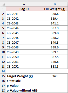
We want to calculate the sample’s t statistic, then turn its magnitude into a valid two-tailed p-value.
First, calculate the t statistic in B16:
=(AVERAGE(B2:B13)-B15)/(STDEV.S(B2:B13)/SQRT(COUNT(B2:B13)))
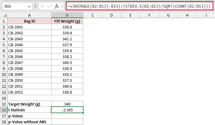
The sample mean is below the target, so the calculation returns a negative t statistic of -2.565.
T.DIST.2T requires a nonnegative x value. The next formula uses ABS to pass the statistic’s magnitude instead of its sign.
=T.DIST.2T(ABS(B16),COUNT(B2:B13)-1)
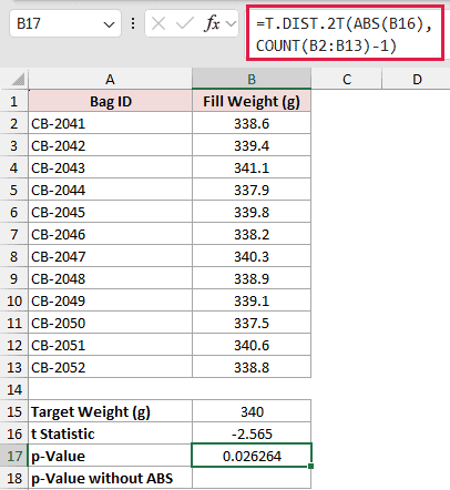
The formula returns 0.026264. It also calculates 11 degrees of freedom by subtracting one from the 12 observations.
The white result cell in B18 deliberately shows what not to do. This formula passes the negative statistic directly to T.DIST.2T:
=T.DIST.2T(B16,COUNT(B2:B13)-1)
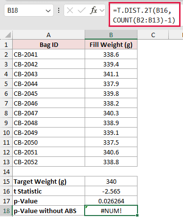
The mistake returns #NUM! because x is negative. Wrapping a calculated t statistic in ABS avoids this problem without changing a two-tailed result.
Example 3: Check a Paired t-Test
Here’s a paired test using scores recorded before and after sales training.
Below is the dataset. Columns B and C contain ten matched score pairs, followed by labeled cells for the t statistic and two p-value methods.
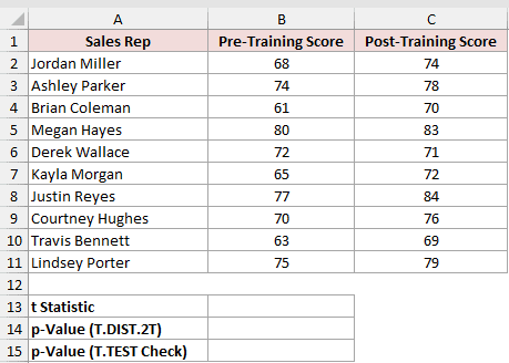
We want the t statistic for the paired differences, its two-tailed p-value, and a T.TEST cross-check.
Use the row-by-row score differences to calculate the paired t statistic:
=AVERAGE(C2:C11-B2:B11)/(STDEV.S(C2:C11-B2:B11)/SQRT(COUNT(B2:B11)))
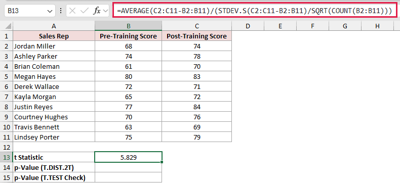
The formula subtracts each pre-training score from its matched post-training score. Their average difference and standard deviation produce a t statistic of 5.829.
Pro Tip: In Excel 2019 and earlier, confirm this range arithmetic formula with Ctrl+Shift+Enter.
Next, convert that statistic to a two-tailed p-value:
=T.DIST.2T(ABS(B13),COUNT(B2:B11)-1)
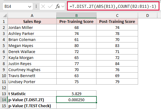
The result is 0.000250 with nine degrees of freedom. Using ABS keeps the formula valid if the average paired difference is negative.
And here is the direct paired T.TEST formula for comparison:
=T.TEST(B2:B11,C2:C11,2,1)
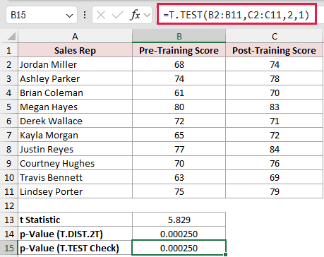
T.TEST also returns 0.000250, confirming the manual route. However, T.TEST returns only the p-value, while this method preserves the t statistic in B13.
Example 4: Calculate Regression p-Values
Next, we’ll rebuild the p-value column for a regression coefficient table.
Below is the dataset. It lists four coefficients and standard errors, with result columns for t statistics, p-values, and significance decisions.
The card below the table holds 22 residual degrees of freedom and an alpha of 0.05.
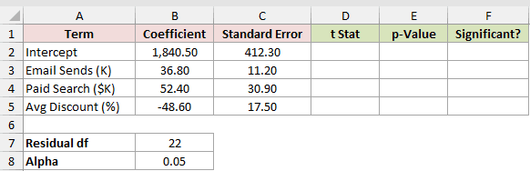
We want to calculate each coefficient’s t statistic, p-value, and significance label with three spilling formulas.
First, divide each coefficient by its standard error:
=B2:B5/C2:C5
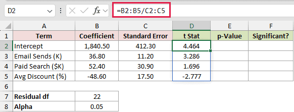
The formula returns four t statistics in D2:D5. The Avg Discount term produces -2.777 because its estimate is negative.
The next formula turns their magnitudes into two-tailed p-values using the residual degrees of freedom in B7:
=T.DIST.2T(ABS(D2:D5),B7)
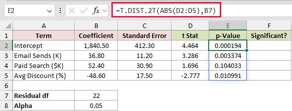
The p-values are 0.000194, 0.003374, 0.104033, and 0.010991. Regression uses residual degrees of freedom, not the usual sample size minus one.
Finally, compare each p-value with the alpha stored in B8:
=IF(E2:E5<B8,"Yes","No")
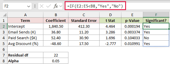
Paid Search is the only term marked No because its p-value of 0.104033 is above 0.05. The other three terms are marked Yes.
The Analysis ToolPak’s Regression tool can produce a static p-value column. This formula-based version recalculates whenever the coefficient or standard error changes.
Example 5: Test From Summary Statistics
Finally, let’s compare two email campaign versions when only summary statistics are available.
Below is the dataset. It contains the order count, average order value, and standard deviation for each version, followed by three labeled result cells.
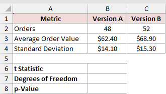
We want a pooled two-sample t statistic, its degrees of freedom, and the resulting two-tailed p-value.
First, calculate the pooled t statistic:
=(C3-B3)/SQRT(((B2-1)*B4^2+(C2-1)*C4^2)/(B2+C2-2)*(1/B2+1/C2))
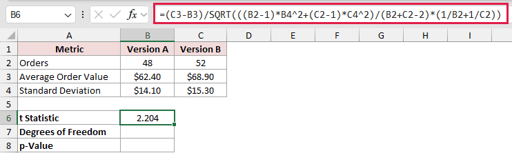
The formula assumes equal population variances. It combines both sample variances and returns a t statistic of 2.204.
Next, calculate the pooled test’s degrees of freedom:
=B2+C2-2
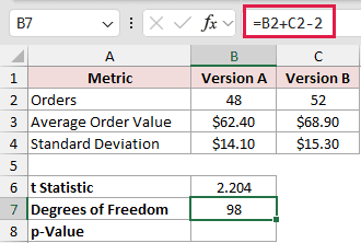
The two sample sizes are 48 and 52, so the formula returns 98 degrees of freedom.
With the statistic and degrees of freedom ready, calculate the two-tailed p-value:
=T.DIST.2T(ABS(B6),B7)
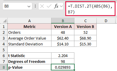
The result is 0.029893. T.TEST cannot calculate this from summary statistics alone because it requires the underlying observation ranges.
If equal variance is not a reasonable assumption, use Welch’s method instead. T.DIST.2T truncates fractional degrees of freedom before calculating the probability.
Tips & Common Mistakes
- T.DIST.2T returns #NUM! when x is negative. Use ABS around a calculated t statistic because a two-tailed probability depends on its magnitude.
- Excel truncates decimal degrees of freedom to an integer. A value below 1 returns #NUM!.
- For a positive t statistic, T.DIST.RT returns the one-tailed right-side probability. The T.DIST.2T result is exactly twice that probability.
- TDIST with its tails argument set to 2 is the legacy equivalent. T.DIST.2T is the current function name and has been available since Excel 2010.
- T.INV.2T performs the inverse operation. It returns the positive t critical value for a two-tailed probability and specified degrees of freedom.
- Both x and deg_freedom can be ranges in the same formula, so you can vary the t statistic and degrees of freedom by row.
T.DIST.2T is most useful once you already have a t statistic and need its two-tailed p-value.
The degrees of freedom must match the test design. For regression results, use residual degrees of freedom rather than sample size minus one.
Related Excel Functions / Articles:
