SERIESSUM Function in Excel

The SERIESSUM function in Excel evaluates a power series using an input value, a starting power, a power step, and a set of coefficients.

It is handy when coefficients already describe a polynomial, approximation, or discounted series. You control which powers Excel uses without writing every term separately.

In this article, I’ll show you how to evaluate calibration and trendline polynomials, approximate SIN and EXP, and calculate NPV.

SERIESSUM Function Syntax in Excel

The SERIESSUM function uses the following syntax:

=SERIESSUM(x, n, m, coefficients)

• x (required) is the input value used in the power series.
• n (required) is the starting power applied to x.
• m (required) is the amount added to the power for each successive coefficient. It can move the powers upward or downward.
• coefficients (required) is the range or array containing the multipliers for the successive powers of x. The number of coefficients sets how many terms the series has.

When to Use SERIESSUM Function

• Evaluate a polynomial when its coefficients are stored in worksheet cells.
• Apply one calibration equation to a column of measurements.
• Reuse coefficients copied from a chart trendline or another Excel calculation.
• Approximate mathematical functions with a finite power series.
• Calculate discounted values when each coefficient represents a cash flow.

Example 1: Evaluate a Calibration Polynomial

Let’s start with a sensor calibration equation.

Below is the dataset. Column A contains voltage readings, the table in columns D and E holds coefficients, and column B will hold the calculated temperatures.

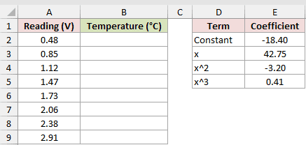
We want to apply the same calibration polynomial to every voltage reading.

Here is the formula entered in B2 and copied down:

=SERIESSUM(A2,0,1,$E$2:$E$5)

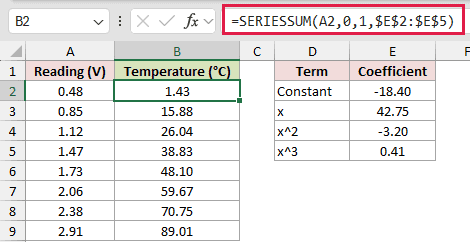
The starting power is 0, so the first coefficient is the constant. The power then increases by 1 for each remaining coefficient.

The absolute reference keeps the coefficient range fixed as the formula is copied down. A reading of 0.48 returns 1.43°C, while 2.91 returns 89.01°C.

SERIESSUM does not accept the entire input column as x. Copying the per-row formula down is the standard way to use SERIESSUM on a column.

Example 2: Use Descending Trendline Coefficients

Here’s a useful setup when a chart equation lists its highest power first.

Below is the dataset. Column A lists vehicle speeds, columns D and E hold descending trendline terms and coefficients, and column B will hold estimated fuel economy.

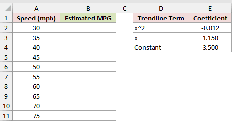
We want to evaluate the trendline without rearranging its coefficients.

Here is the formula entered in B2 and copied down:

=SERIESSUM(A2,2,-1,$E$2:$E$4)

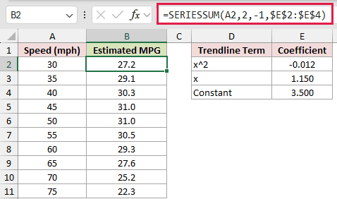
The formula begins with power 2 and uses a step of -1. That matches the coefficient order: squared term, linear term, then constant.

At 30 mph, the equation returns 27.2 MPG. At 50 mph, it returns 31.0 MPG, and at 75 mph it returns 22.3 MPG.

Pro Tip: Check the coefficient order before choosing n and m. LINEST also returns polynomial coefficients with the highest power first, so a negative step can preserve that order.

Example 3: Approximate SIN With Odd Powers

Now let’s see how the power step can skip unwanted exponents.

Below is the dataset. Column A contains angles, columns E and F hold odd-power coefficients, and columns B and C will hold the series estimate and SIN result.

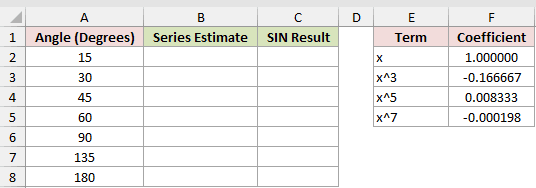
We want to approximate each sine value using the coefficient table.

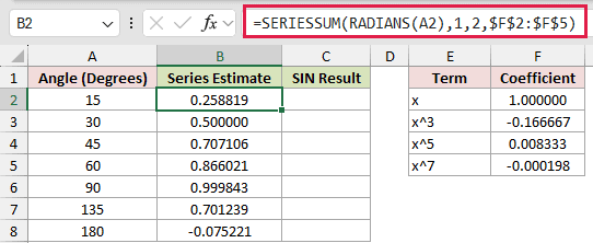
Here is the SERIESSUM formula entered in B2 and copied down:

=SERIESSUM(RADIANS(A2),1,2,$F$2:$F$5)

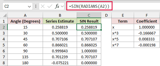
And here is the built-in SIN formula entered in C2 and copied down:

=SIN(RADIANS(A2))

Starting at power 1 and stepping by 2 selects the odd powers shown in the coefficient table.

At 15 degrees, both columns display 0.258819. At 90 degrees, the estimate is 0.999843 while SIN displays 1.000000.

The approximation becomes less accurate farther from zero. At 180 degrees, the series returns -0.075221 while SIN displays 0.000000.

That displayed SIN value is rounded by the cell format. It does not mean the underlying SIN calculation returns exactly zero.

Example 4: Vary the Number of Terms

Let’s build the coefficient array instead of typing every coefficient.

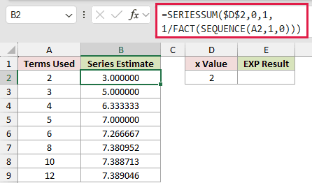
Below is the dataset. Column A lists the term counts, D2 contains the x value, and columns B and E will hold the series estimates and EXP check.

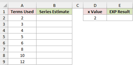
We want to see how the estimate changes as the coefficient array grows.

Here is the SERIESSUM formula entered in B2 and copied down:

=SERIESSUM($D$2,0,1,1/FACT(SEQUENCE(A2,1,0)))

And here is the EXP formula used as the check:

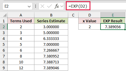
=EXP(D2)

SEQUENCE starts at 0 and creates the required number of positions. FACT converts them to factorials, and 1/ turns each factorial into its reciprocal.

The coefficients are therefore 1/0!, 1/1!, 1/2!, and so on, which form the series for EXP. SERIESSUM evaluates that calculated array.

With 2 terms, the estimate is 3.000000. With 12 terms, it reaches 7.389046, close to the EXP result of 7.389056.

SEQUENCE requires Excel 2021 or later for this setup. In earlier versions, place the coefficients in cells and pass that range to SERIESSUM.

Example 5: Calculate NPV With Year Zero

Finally, let’s use a power series to discount project savings.

Below is the dataset. Columns A and B contain project years and net savings, while the card holds the discount rate and two labeled NPV result cells.

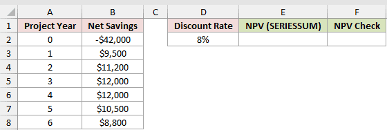
We want to discount every cash flow while keeping the Year 0 cost undiscounted.

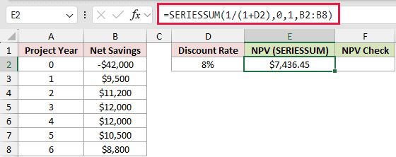
Here is the SERIESSUM formula:

=SERIESSUM(1/(1+D2),0,1,B2:B8)

And here is the NPV formula used as the check:

=NPV(D2,B3:B8)+B2

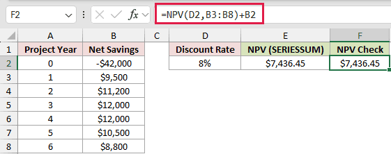
The x argument becomes the discount factor. Starting at power 0 leaves the Year 0 value unchanged. Each later cash flow receives another discounting step.

Both formulas return $7,436.45. The NPV check adds B2 separately because Excel’s NPV function discounts every value it receives, including the first, by at least one period.

Including B2 inside NPV would discount the Year 0 cost by a full year, so the formula adds B2 undiscounted.

Tips & Common Mistakes

• SERIESSUM does not spill when you pass a range to x. Enter the first-row formula and copy it down for ordinary worksheet tables.
• In Microsoft 365 and Excel 2024, MAP with LAMBDA can apply SERIESSUM to each input and return a spilled column.
• Do not leave gaps inside a coefficient range. In testing, coefficients 1, blank, and 3 at x=2 returned 7 because the blank was skipped. Enter 0 instead.
• A text value inside the coefficient range returns #VALUE!. Check imported coefficients before using them in a series.
• Match n and m to the coefficient order. Coefficients for ascending powers need a positive m, while coefficients for descending powers need a negative m.
• Use a built-in function as a check when you are approximating a known mathematical result. Display formatting can hide a small difference.

I covered how SERIESSUM evaluates calibration and trendline polynomials, approximates SIN and EXP, and discounts project cash flows for an NPV calculation.

I hope you found this article helpful.

List of All Excel Functions

Related Excel Functions / Articles:

• POWER Function in Excel
• LOGEST Function in Excel
• How to Sum a Column in Excel?