If you want to generate a list of numbers, dates, or any evenly spaced series in Excel without dragging a fill handle, the SEQUENCE function in Excel is the cleanest way to do it.
SEQUENCE is a native dynamic array function. You enter one formula, and the result spills automatically into the cells below or beside it.
There’s no Ctrl+Shift+Enter, no helper columns, and no fill handle. In this article, I’ll walk you through the four arguments SEQUENCE takes and a handful of practical examples you can adapt to your own work.
One thing worth flagging up front. SEQUENCE only ships in Excel for Microsoft 365, Excel 2021/2024, and Excel for the web. If you’re on Excel 2019 or earlier, you won’t have this function.
SEQUENCE Function Syntax
Here is the syntax of the SEQUENCE function:
=SEQUENCE(rows, [columns], [start], [step])
- rows – The number of rows you want in the output. This is the only required argument.
- columns – Optional. The number of columns you want in the output. Defaults to 1.
- start – Optional. The first number in the sequence. Defaults to 1.
- step – Optional. The amount to add to each successive number. Defaults to 1. Can be negative for a descending series.
The result spills into adjacent cells automatically, so you only enter the formula once and Excel sizes the output for you.
When to Use SEQUENCE
Use this function when you need to:
- Generate a list of row numbers or sequential numbers in Excel without dragging
- Build a list of consecutive dates, months, or years
- Create a 2D grid of numbers (multiplication tables, fixture grids, calendar layouts)
- Feed an array of indexes into another function (INDEX, FILTER, TEXT, EDATE, EOMONTH, CHAR)
- Quickly produce a numbered list of any length, even 10,000 rows
Let me show you a few practical examples of how to use this function.
Example 1: Generate Numbers 1 to 10
Let’s start with the simplest case. I want a list of numbers from 1 to 10 in a single column.
Here is the formula:
=SEQUENCE(10)

In the above formula, only the rows argument is supplied. Columns defaults to 1, start defaults to 1, and step defaults to 1, so you get 1 through 10 stacked in a column.
If you want to change how many numbers come out, just change that first argument. =SEQUENCE(100) gives you 1 to 100.
Example 2: Build a Row Instead of a Column
Now let’s flip the orientation. I want the same numbers, but going across the row instead of down a column.
Here is the formula:
=SEQUENCE(1,10)
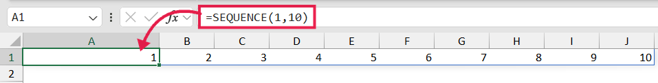
Here, I’m asking for 1 row and 10 columns. The output spills horizontally instead of vertically.
This is handy when you need column headers like Episode 1, Episode 2, Episode 3, and so on. Wrap it in a quick text formula and you’ve got dynamic headers that update if you change the count.
Example 3: Custom Start and Step
What if you don’t want to start at 1?
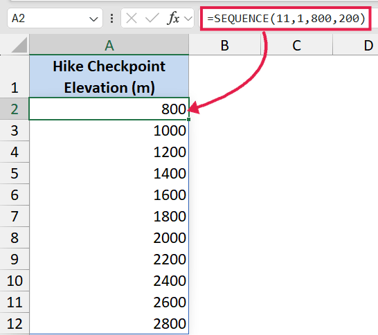
Let’s say I’m logging hike checkpoints every 200 meters from 800 meters to 2,800 meters of elevation.
I want SEQUENCE to spill that list of checkpoint elevations into the cells below.
Here is the formula:
=SEQUENCE(11,1,800,200)
How this formula works:
- 11 tells SEQUENCE to return 11 rows.
- 1 is the column count (one column).
- 800 is the starting elevation in meters.
- 200 is the step, so each checkpoint sits 200 m above the previous one.
You can also flip the direction by passing a negative step. For a descending altimeter readout, =SEQUENCE(11,1,2800,-200) gives you 2800, 2600, 2400, all the way down to 800.
Pro Tip: If you’re not sure how many rows you need to land on a target end value, use this pattern. =SEQUENCE((end-start)/step+1, 1, start, step). So for 800 to 2800 in steps of 200, that’s (2800-800)/200+1 = 11 rows.
Example 4: Generate a List of Dates
Because Excel stores dates as serial numbers, SEQUENCE works great for date series too.
Here I want the next 14 days starting today, for a content-publishing schedule.
Here is the formula:
=SEQUENCE(14,1,TODAY(),1)
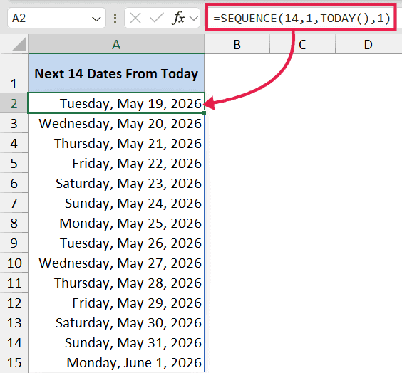
In the above formula, TODAY() gives the start date as a serial number, and SEQUENCE adds 1 each row to produce the next 14 dates.
The output will look like serial numbers at first. Just format the result range as a date and you’re done.
The same pattern handles months and end-of-month dates beautifully. =EOMONTH(TODAY(), SEQUENCE(12,1,0)) spills the next 12 month-ends from today, which is the cleanest one-formula way to build a quarterly or annual reporting calendar.
If you want to learn other ways to fill a date column without SEQUENCE, here’s a separate guide on how to autofill dates in Excel, and another on how to list all dates between two dates using a few different approaches.
Example 5: Build a Round-Robin Fixture Grid
This one shows off the 2D power of SEQUENCE.
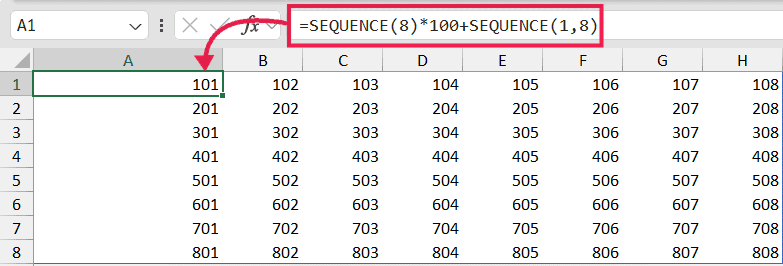
Say I’m setting up an 8-team round-robin tournament and want a fixture-ID grid where the row is the home team number and the column is the away team.
Each cell encodes the matchup as home*100 + away, so home team 3 versus away team 7 reads as 307.
Here is the formula:
=SEQUENCE(8)*100+SEQUENCE(1,8)
How this formula works:
SEQUENCE(8)produces a vertical 1-8 column for the home teams.SEQUENCE(1,8)produces a horizontal 1-8 row for the away teams.- Multiplying the vertical by 100 and adding the horizontal pairs every home team with every away team and returns an 8×8 grid of fixture codes (101, 102, 103… up to 808).
That’s broadcasting in action: a vertical array combined with a horizontal array fans out into a rectangle.
The same trick works anywhere you need every-row-against-every-column. Multiplication tables, distance matrices, calendar layouts, and pricing grids all fall out of the same pattern.
Example 6: SEQUENCE Inside Other Dynamic Arrays
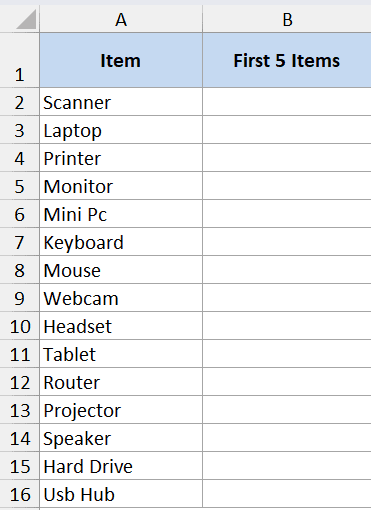
SEQUENCE really shines when you nest it inside other functions. Here’s a quick one. I want the first 5 items from a list in column A.
Here is the formula:
=INDEX(A2:A100, SEQUENCE(5))
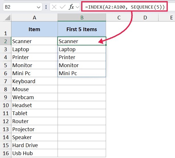
INDEX normally returns one value, but when you feed it an array of row numbers from SEQUENCE, it returns all of those rows at once and spills the result.
You can do similar tricks with TEXT (for formatted dates), CHAR (for letter sequences via CHAR(SEQUENCE(26,1,65)) to spill A through Z), or wrap SEQUENCE inside SORT and FILTER for paginated views of a dataset.
Tips & Common Mistakes
- #SPILL! error – If the cells where SEQUENCE wants to spill aren’t empty, you’ll get a #SPILL! error in Excel. Clear the cells in the spill range or move the formula to a clear area.
- The
#operator references the whole spill – If your SEQUENCE lives in cellD2, refer to its full output asD2#in any downstream formula. The reference resizes automatically when you change the rows or columns argument, so charts and summary formulas built onD2#always track the live output. - Watch for the
@implicit intersection – If a workbook gets saved by an older Excel version, an@symbol can sneak in in front of your formula (=@SEQUENCE(10)), which collapses the spill to a single cell. Delete the@and the spill comes back. - Not available in older Excel – SEQUENCE was rolled out with the dynamic array engine. If you’re on Excel 2019, 2016, or earlier, the function simply doesn’t exist. Microsoft 365 or Excel 2021 is the minimum.
- Don’t wrap SEQUENCE in
{}array braces – It’s already a dynamic array, not one of the old array formulas in Excel. Just press Enter normally. No Ctrl+Shift+Enter needed (and no, you can’t make it spill in Excel 2019 by adding CSE either). - Format the output for dates – When you generate a date series, the cells will show 5-digit serial numbers until you format them as dates. The numbers are correct, the formatting just needs to catch up.
- Negative step works fine – For descending series, just pass a negative number.
=SEQUENCE(5,1,10,-2)gives you 10, 8, 6, 4, 2. - Decimal step works too – You’re not limited to whole numbers.
=SEQUENCE(5,1,0,0.25)gives you 0, 0.25, 0.5, 0.75, 1.
That’s the SEQUENCE function in Excel. It’s one of those small dynamic-array additions that quietly replaces a lot of fill-handle dragging and helper columns.
Once you start using it, you’ll spot places it fits everywhere, especially anywhere you need a clean array of numbers, dates, or grid coordinates without manually building the list.
Related Excel Functions / Articles: