
Excel’s ACOTH function returns the inverse hyperbolic cotangent of a real number whose absolute value is greater than 1.
That creates two valid input regions: numbers below -1 and numbers above 1. The result keeps the input’s sign.
In this article, I’ll show you how to calculate signed results, reverse COTH values, validate imported data, and audit the formula.
ACOTH Function Syntax in Excel
The ACOTH function has one required argument:
=ACOTH(number)
numberis a real number with an absolute value greater than 1.
When to Use ACOTH Function
- Reverse a value produced by the COTH function
- Calculate inverse hyperbolic cotangents for positive and negative inputs
- Validate imported values against ACOTH’s two-part domain
- Compare Excel’s result with the equivalent logarithmic expression
Example 1: Calculate Signed ACOTH Results
Let’s start with valid inputs on both sides of the excluded interval.
The dataset has calculation IDs in column A, valid signed inputs in column B, and an empty ACOTH result column in C.
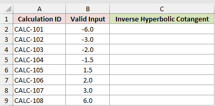
I want one inverse hyperbolic cotangent for every value in B2:B9.
Here is the formula:
=ACOTH(B2:B9)
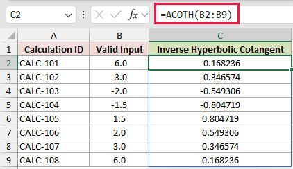
The formula starts in C2 and spills through C9. Negative inputs return negative results, while positive inputs return positive results.
For example, -2 returns approximately -0.549306 and 2 returns approximately 0.549306.
In Excel 2021, Excel 2024, and Microsoft 365, entering the range formula once fills the results automatically.
Pro Tip: Keep C2:C9 clear before entering the formula. A value blocking the intended output range causes a #SPILL! error.
Example 2: Reverse COTH Results
This example checks ACOTH against its companion function.
The dataset lists signed parameters in column B. Columns C and D hold the COTH output and the value recovered with ACOTH.
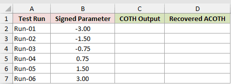
I want to calculate COTH for each nonzero parameter, then recover that original parameter.
Here is the COTH formula:
=COTH(B2:B7)
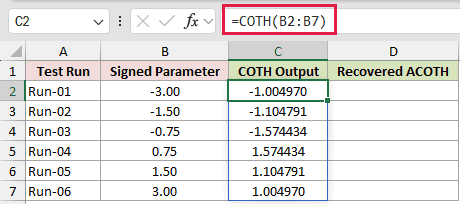
COTH returns values outside the closed interval from -1 through 1, so every result in column C is valid for ACOTH.
Now reverse those values with ACOTH:
=ACOTH(C2:C7)
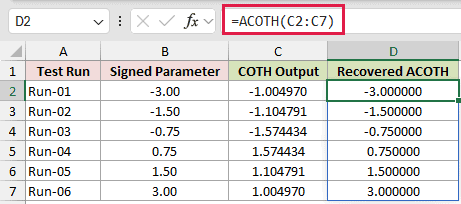
Column D recovers the signed inputs from column B. Small floating-point differences may appear in unrounded cells, such as -3.000000000000017 instead of exactly -3.
The worksheet displays six decimal places, so those tiny calculation differences do not change the shown values.
Example 3: Validate Inputs Before ACOTH
Imported values can fall inside ACOTH’s excluded interval.
The dataset has import IDs in column A, incoming values in column B, and an empty checked-result column in C.
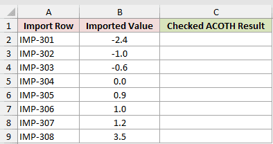
I want valid inputs calculated and every value from -1 through 1 flagged.
Here is the formula:
=IF(ABS(B2:B9)>1,ACOTH(B2:B9),"Outside domain")
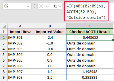
ABS measures each input’s distance from zero. IF runs ACOTH only when that distance is greater than 1.
Values such as -1, 0, and 1 return “Outside domain.” Valid inputs, including -2.4 and 1.2, return their ACOTH results.
Without the domain check, a value whose absolute value is 1 or less returns #NUM!.
Pro Tip: Test ABS(number)>1. A check such as number>1 would incorrectly reject valid negative inputs below -1.
Example 4: Audit the ACOTH Calculation
The logarithmic form makes a useful independent check.
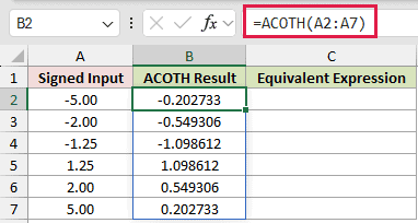
The dataset lists signed inputs in column A. Columns B and C hold the built-in ACOTH result and the equivalent expression.
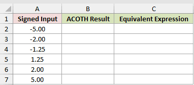
I want to compare Excel’s ACOTH results with the underlying logarithmic calculation.
First, calculate the built-in results:
=ACOTH(A2:A7)
Now calculate the equivalent expression:
=0.5*LN((A2:A7+1)/(A2:A7-1))
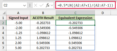
The two columns match to the worksheet’s six displayed decimal places. For -2, both formulas return approximately -0.549306.
ACOTH is clearer for everyday work. The logarithmic expression is useful when an audit requires the underlying calculation or an older Excel version lacks ACOTH.
Tips & Common Mistakes
- ACOTH requires
ABS(number)>1. The boundary values -1 and 1 are invalid, along with every value between them. - ACOTH is the inverse hyperbolic cotangent. ACOT handles the ordinary circular cotangent and follows different input and result rules.
- ACOTH returns a hyperbolic value, not a conventional circular angle. Converting it with DEGREES would give a misleading interpretation.
- ACOTH was introduced in Excel 2013. Earlier Excel versions can use the equivalent logarithmic expression for valid inputs.
- Range formulas spill in Excel 2021, Excel 2024, and Microsoft 365. Older versions need per-row formulas or legacy array entry.
- There is no newer direct replacement for ACOTH.
I covered signed ACOTH results, COTH reversal, domain checks, and an equivalent logarithmic calculation.
I hope you found this article helpful.
Other Excel articles you may also like:
