
Excel’s BETA.DIST function returns either the cumulative probability or probability density for a beta distribution.
The beta distribution models values within fixed limits. It works especially well for rates, proportions, and task durations that can’t fall outside a defined range.
In this article, I’ll show you how to compare probability with density, find the chance between two values, and estimate probabilities from counts and historical data.
BETA.DIST Function Syntax in Excel
BETA.DIST needs a value, two shape parameters, and a cumulative setting, with optional lower and upper bounds.
=BETA.DIST(x,alpha,beta,cumulative,[A],[B])
- x (required) is the value between A and B, inclusive, where you want to evaluate the distribution. The default range is 0 to 1.
- alpha (required) is the first shape parameter and must be greater than zero.
- beta (required) is the second shape parameter and must be greater than zero.
- cumulative (required) is TRUE for the cumulative probability or FALSE for the probability density.
- A (optional) is the lower bound. Excel uses 0 when you omit it.
- B (optional) is the upper bound. Excel uses 1 when you omit it.
Alpha and beta can be decimals. Changing their relative sizes changes the distribution’s shape and where its values concentrate.
When to Use BETA.DIST Function
- Find the chance that a rate or proportion is at most a chosen value.
- Calculate the chance that a value falls within a specific band.
- Compare a measured success rate with a target after accounting for the number of observations.
- Estimate the chance that a task finishes within a budgeted duration.
- Model historical rates after estimating alpha and beta from their average and variance.
Example 1: Compare Cumulative Probability and Density
Let’s start by comparing the function’s two calculation modes.
Below is the dataset. Column A lists completion rates. Columns B and C have green result headers and empty cells, while E:F holds Alpha 4 and Beta 6.
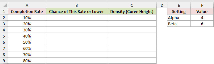
We want the cumulative chance and density for every listed completion rate.
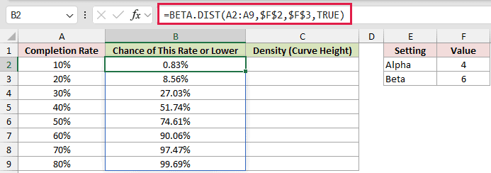
Here is the cumulative formula:
=BETA.DIST(A2:A9,$F$2,$F$3,TRUE)
And here is the density formula:
=BETA.DIST(A2:A9,$F$2,$F$3,FALSE)
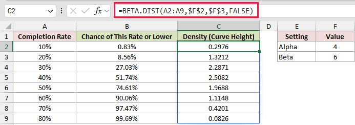
At 40%, the cumulative formula returns 51.74%. This means the modeled chance of a completion rate at or below 40% is 51.74%.
The density formula returns 2.5082 at 40%. That number is the curve’s height, not a probability, so a density can be greater than 1.
Both formulas spill in Excel 2021, Excel 2024, and Microsoft 365. In Excel 2019 or earlier, enter a single-row version and fill it down.
Example 2: Find Probability Between Two Values
Here’s a practical way to calculate the chance within several bands.
Below is the dataset. It lists five email open-rate bands with lower and upper limits.
The Chance of Landing in Band header is green, with empty bordered cells below. G2:G3 holds Alpha 22 and Beta 58.
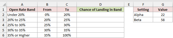
We want the modeled chance that the open rate lands inside each band.
Here is the formula:
=BETA.DIST(C2:C6,$G$2,$G$3,TRUE)-BETA.DIST(B2:B6,$G$2,$G$3,TRUE)
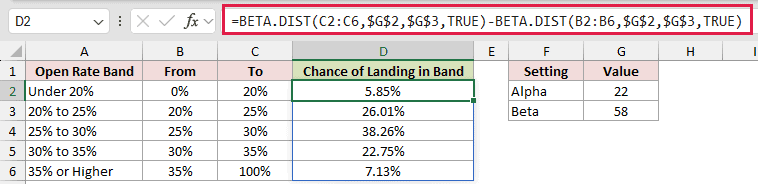
Each row subtracts the cumulative probability at the lower limit from the cumulative probability at the upper limit.
The 25% to 30% band returns 38.26%, the largest chance in the table. All five band results add to 100%.
Because this is a continuous distribution, you don’t subtract 1 from either boundary as you might with discrete counts.
Example 3: Test Whether a Rate Beats a Target
Now let’s use purchase counts to judge several campaign rates.
Below is the dataset. It lists campaigns, clicks, and purchases. Observed Rate and Chance True Rate Beats Target are green headers with empty bordered cells below.
The 4% target rate is in H2.
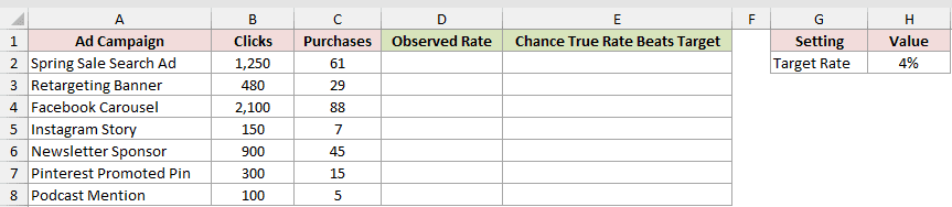
We want each observed purchase rate and the modeled chance that its true rate exceeds 4%.
First, calculate the observed rates:
=C2:C8/B2:B8
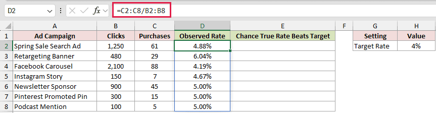
Then calculate the chance that each true rate beats the target:
=1-BETA.DIST($H$2,C2:C8+1,B2:B8-C2:C8+1,TRUE)
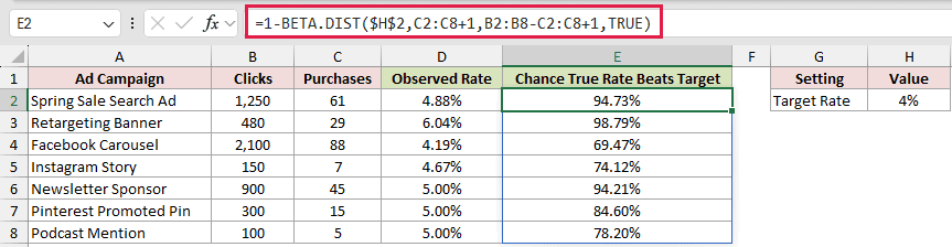
The second formula uses purchases plus 1 as alpha. It uses non-purchases plus 1 as beta, then subtracts the target’s cumulative probability from 1.
The added 1s come from starting with a flat assumption. Before seeing any data, every rate from 0% to 100% is treated as equally likely.
The Newsletter Sponsor, Pinterest Promoted Pin, and Podcast Mention each show a 5.00% observed rate.
The modeled chances are 94.21%, 84.60%, and 78.20% for Newsletter Sponsor, Pinterest Promoted Pin, and Podcast Mention, respectively.
More observations produce stronger evidence even when the observed rates match.
Example 4: Estimate PERT Task Completion Chances
Let’s move from proportions to task durations measured in days.
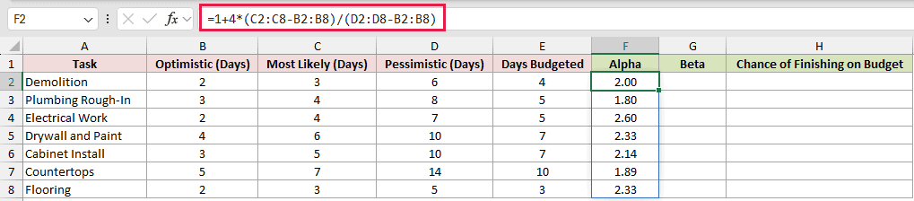
Below is the dataset. It lists seven remodel tasks with optimistic, most likely, pessimistic, and budgeted durations.
The Alpha, Beta, and Chance of Finishing on Budget headers are green, with empty bordered cells below them.

We want PERT shape parameters and the chance that each task finishes within its budget.
First, calculate alpha:
=1+4*(C2:C8-B2:B8)/(D2:D8-B2:B8)
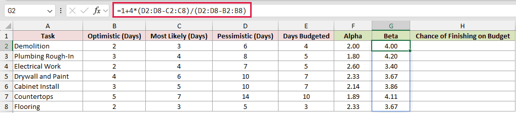
Next, calculate beta:
=1+4*(D2:D8-C2:C8)/(D2:D8-B2:B8)
Now calculate each on-budget chance:
=BETA.DIST(E2:E8,F2:F8,G2:G8,TRUE,B2:B8,D2:D8)
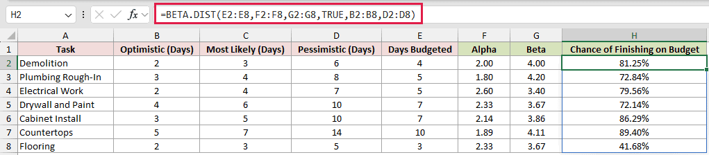
The alpha and beta formulas turn each three-point estimate into shape parameters. BETA.DIST then uses the optimistic and pessimistic durations as its A and B bounds.
Flooring has a 41.68% chance of finishing within its three-day budget. Budgeting the most likely duration doesn’t automatically create a 50% chance.
Countertops returns 89.40% for its ten-day budget, the highest chance in this table.
Example 5: Fit BETA.DIST From Historical Rates
Sometimes you have past rates but no ready-made alpha and beta values.
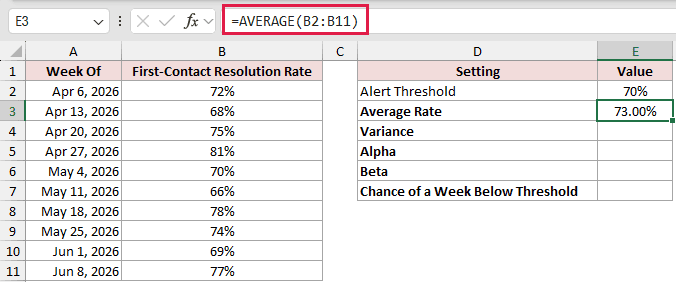
Below is the dataset. It lists ten weekly resolution rates beside a settings card.
The card has a filled 70% Alert Threshold in E2. E3:E7 are empty for Average Rate, Variance, Alpha, Beta, and Chance of a Week Below Threshold.
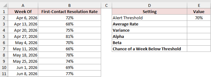
We want to fit alpha and beta from the history, then estimate the chance of a week at or below 70%.
First, calculate the average rate:
=AVERAGE(B2:B11)
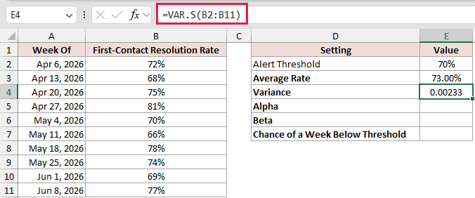
Next, calculate the sample variance:
=VAR.S(B2:B11)
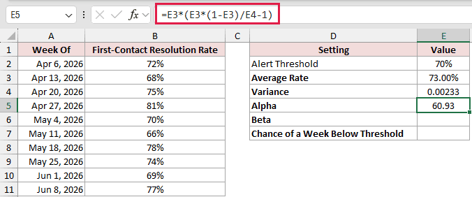
Use those two results to calculate alpha:
=E3*(E3*(1-E3)/E4-1)
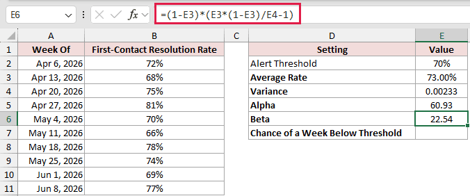
Then calculate beta:
=(1-E3)*(E3*(1-E3)/E4-1)
Finally, calculate the chance of falling below the alert threshold:
=BETA.DIST(E2,E5,E6,TRUE)
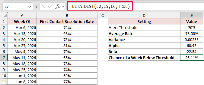
The weekly rates have an average of 73.00% and a variance of 0.00233. The fitted alpha and beta values are 60.93 and 22.54.
BETA.DIST returns 26.11%, so the fitted model assigns about a one-in-four chance to a week at or below the 70% threshold.
Example 6: Diagnose BETA.DIST #NUM! Errors
The last example puts valid inputs and common failures side by side.
Below is the dataset. The Scenario column labels each row, alongside x, Alpha, Beta, Lower Bound (A), and Upper Bound (B) columns.
The Result header is green, and the bordered cells below it are empty.
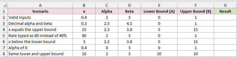
We want to see which rows return cumulative probabilities and which return #NUM!.
Here is the formula:
=BETA.DIST(B2:B8,C2:C8,D2:D8,TRUE,E2:E8,F2:F8)
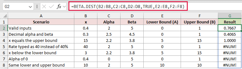
The valid row returns 0.7667, and decimal shape parameters return 0.4065. When x equals the upper bound, the cumulative result is 1.0000.
Typing 40 instead of 40% places x outside the 0 to 1 bounds, so Excel returns #NUM!.
Excel also returns #NUM! when x is below A, alpha is zero, or A and B are equal.
The spilled formula evaluates each row separately. Valid rows still return numbers when other rows contain errors.
Tips & Common Mistakes
- The cumulative argument is required. Leaving it out causes Excel to reject the formula at entry.
- A blank cumulative cell acts as FALSE and returns density. Use an explicit TRUE or FALSE to avoid a silent wrong result.
- If you omit A and B, Excel uses 0 and 1. Supplying only A leaves B at 1, so enter both bounds when scaling the distribution.
- Excel returns #NUM! when x falls outside the bounds, alpha or beta is zero or negative, or A is not less than B.
- Cumulative calculations allow x to equal A or B. A density calculation can return #NUM! at a bound when the corresponding shape parameter is below 1.
- Keep the cells beneath a spilling formula empty. Otherwise, Excel returns #SPILL! instead of the expected results.
- The older BETADIST function is retained for compatibility and always returns a cumulative result. Use BETA.DIST for new work.
- Use BETA.INV for the reverse problem when you know the desired probability and need the corresponding value.
With BETA.DIST, you can compare cumulative probability with density, find band chances, model rates from counts, and estimate PERT completion chances.
You can also fit alpha and beta from historical rates and trace #NUM! errors to invalid shapes, bounds, or x values.
Related Excel Functions / Articles:
