
Excel’s BETA.INV function returns the value at a specified cumulative probability for a beta distribution.
It’s useful when a quantity has known lower and upper limits but may be skewed within that range.
In this article, I’ll show you how to calculate bounded percentiles, estimate project durations, compare uncertain rates, and run a release simulation.
BETA.INV Function Syntax in Excel
The BETA.INV function accepts a probability, two shape parameters, and optional lower and upper bounds.
=BETA.INV(probability,alpha,beta,[A],[B])
- probability (required) is the cumulative probability associated with the value you want. It must be greater than 0 and less than 1.
- alpha (required) is the first positive shape parameter of the beta distribution.
- beta (required) is the second positive shape parameter of the beta distribution.
- A (optional) is the lower bound of the distribution. Excel uses 0 when you omit it.
- B (optional) is the upper bound of the distribution. Excel uses 1 when you omit it, and B must be greater than A.
The older BETAINV function returns the same result, but BETA.INV is the current function name.
When to Use BETA.INV Function
- Convert cumulative probabilities into percentiles of a beta distribution.
- Turn bounded three-point estimates into P50, P80, or P95 durations.
- Calculate a credible range for an uncertain rate from event counts.
- Rank products using a conservative score that accounts for sample size.
- Generate bounded random values for a simulation.
Example 1: Spill Beta Distribution Percentiles
Let’s start with a standard beta distribution bounded between 0 and 1.
Below is the dataset. Column A holds seven probabilities, and column B has a green result header with empty cells. The settings card contains alpha and beta.
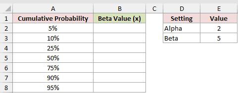
The next step is to calculate one beta value for each probability in column A.
Here is the formula entered in B2:
=BETA.INV(A2:A8,$E$2,$E$3)
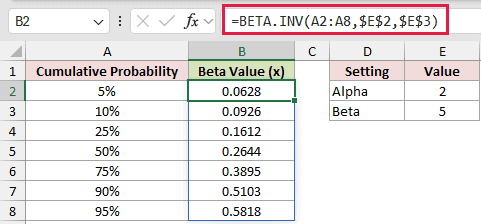
The formula uses alpha 2 and beta 5, then spills seven results from B2 through B8.
The 5% probability returns 0.0628, the 50% probability returns 0.2644, and the 95% probability returns 0.5818.
Range-based BETA.INV formulas spill in Excel 2021, Excel 2024, and Microsoft 365. In Excel 2019 and earlier, enter a single-row formula and fill it down.
Pro Tip: Keep B2:B8 empty before entering the formula. A blocked output range returns #SPILL!.
Example 2: Calculate PERT Approval Percentiles
Here’s a bounded estimate for a city permit approval.
Below is the dataset. Column A lists five confidence levels, and the green cells in column B are empty. The card holds three estimates with empty alpha and beta cells.
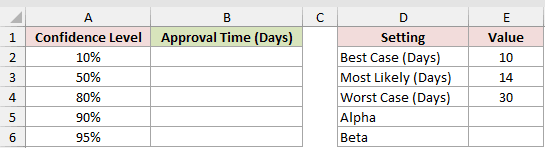
We first need shape parameters from the best, most likely, and worst-case estimates.
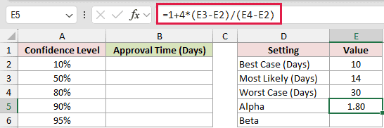
Here is the alpha formula in E5:
=1+4*(E3-E2)/(E4-E2)
And here is the beta formula in E6:
=1+4*(E4-E3)/(E4-E2)
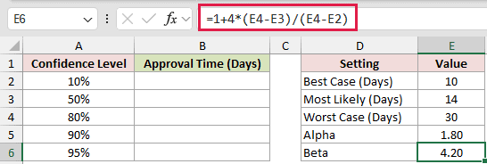
Alpha returns 1.80, while beta returns 4.20. The formulas apply the standard PERT weighting of four to the most likely estimate.
We can now calculate the approval-time percentiles in days.
Here is the formula entered in B2:
=BETA.INV(A2:A6,$E$5,$E$6,$E$2,$E$4)
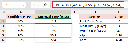
The optional A and B arguments scale the distribution between the best case of 10 days and the worst case of 30 days.
The most likely estimate is 14 days in E3, but the P50 is 15.5 days and the P95 is 22.4 days.
The long tail points toward the 30-day worst case.
Example 3: Calculate Feature P50 and P80
Let’s apply the same PERT approach across a software release plan.
Below is the dataset. Each feature has best, most likely, and worst-case durations. The four green columns contain empty cells for alpha, beta, P50, and P80.

We’ll calculate a separate alpha and beta pair for each feature.
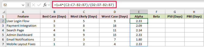
Here is the alpha formula entered in E2:
=1+4*(C2:C7-B2:B7)/(D2:D7-B2:B7)
And here is the beta formula entered in F2:
=1+4*(D2:D7-C2:C7)/(D2:D7-B2:B7)
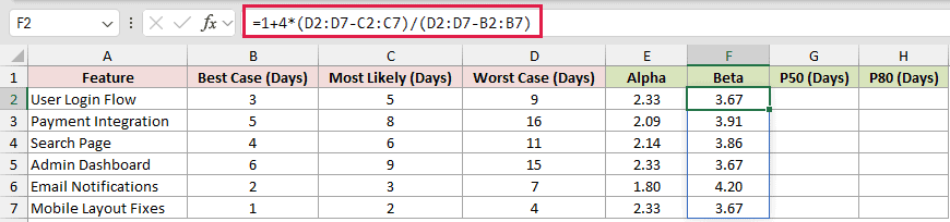
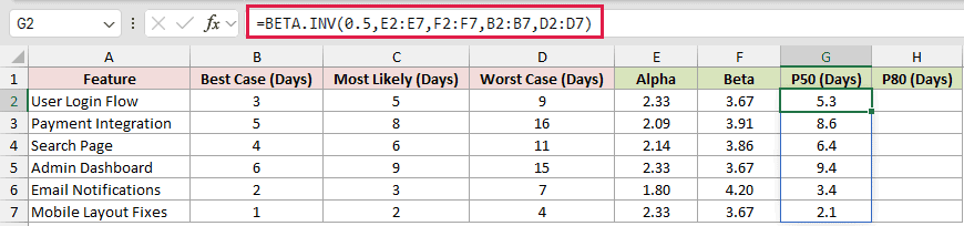
Each feature row gets alpha and beta values from its three estimates. For example, User Login Flow gets 2.33 and 3.67.
Next, the median duration for each feature goes in column G.
Here is the P50 formula entered in G2:
=BETA.INV(0.5,E2:E7,F2:F7,B2:B7,D2:D7)
A more cautious P80 duration goes in column H.
Here is the P80 formula entered in H2:
=BETA.INV(0.8,E2:E7,F2:F7,B2:B7,D2:D7)
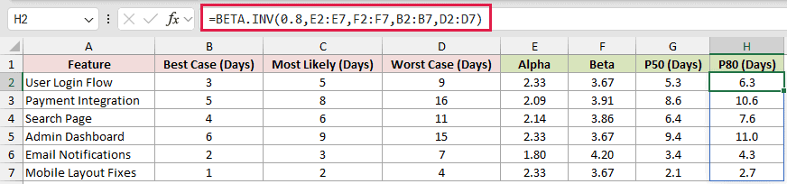
BETA.INV evaluates the alpha, beta, lower-bound, and upper-bound arrays row by row. Each formula returns six results from one entry cell.
For the User Login Flow, the P50 is 5.3 days and the P80 is 6.3 days. Payment Integration moves from 8.6 to 10.6 days.
The P50 to P80 gap differs by feature because each feature’s range and skew differ.
User Login Flow moves from 5.3 to 6.3 days, while Payment Integration moves from 8.6 to 10.6 days.
Example 4: Estimate a Return Rate Range
Here’s a practical way to describe uncertainty around product return rates.
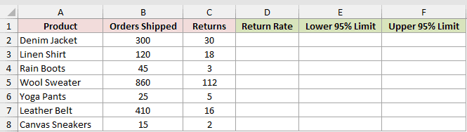
Below is the dataset. It lists products, shipped orders, and returns. The three green columns have empty cells for the observed rate and its lower and upper limits.
We’ll start by calculating each product’s observed return rate.
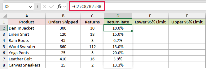
Here is the formula entered in D2:
=C2:C8/B2:B8
Next, we’ll calculate the lower limit of each product’s 95% credible interval.
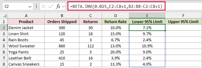
Here is the lower-limit formula entered in E2:
=BETA.INV(0.025,C2:C8+1,B2:B8-C2:C8+1)
The matching upper limits go in column F.
Here is the upper-limit formula entered in F2:
=BETA.INV(0.975,C2:C8+1,B2:B8-C2:C8+1)
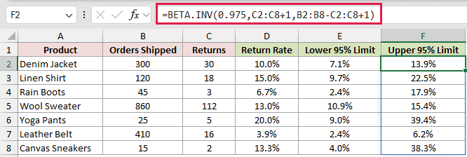
The +1 terms apply a flat starting prior to the return and non-return counts. The result is a Bayesian credible interval, not a classical confidence interval.
The Denim Jacket has a 10.0% observed rate and a 7.1% to 13.9% range.
The Wool Sweater and Canvas Sneakers have close observed rates of 13.0% and 13.3%.
The sweater’s 10.9% to 15.4% range is far narrower because it has 860 orders, compared with 15 for the sneakers.
Example 5: Rank Products Conservatively
Small samples can make a perfect rating look more certain than it is.
Below is the dataset. Columns B and C contain thumbs-up and thumbs-down counts. The two green columns have empty cells for positive share and conservative score.
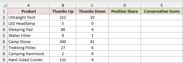
First, we’ll calculate each product’s raw positive share in column D.
Here is the formula entered in D2:
=B2:B9/(B2:B9+C2:C9)
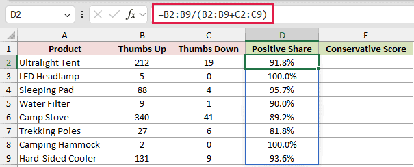
Then we’ll calculate a cautious score from the fifth percentile of each modeled positive rate.
Here is the conservative-score formula entered in E2:
=BETA.INV(0.05,B2:B9+1,C2:C9+1)
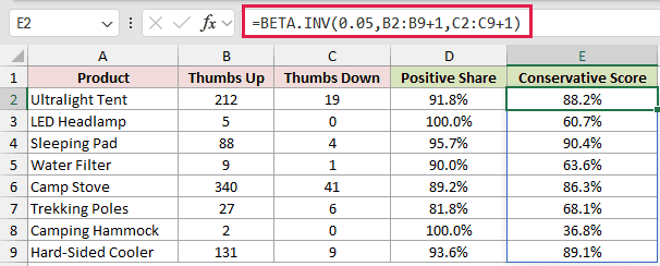
The LED Headlamp and Camping Hammock both have a 100.0% positive share. Their conservative scores fall to 60.7% and 36.8% because their samples are small.
The Sleeping Pad leads on the conservative score at 90.4%, followed by the Hard-Sided Cooler at 89.1%.
In Excel 2021 or later, =SORTBY(A2:A9,E2:E9,-1) can return the product names in conservative-score order. The helper columns still make the ranking logic easy to inspect.
Example 6: Simulate a Release P80
Now let’s estimate the release duration when feature times vary independently.
Below is the dataset. Columns B to D hold each feature’s best-case, most likely, and worst-case days.
The feature table has empty alpha, beta, and simulated-day cells. The card holds 2,000 runs and two empty P80 result cells.

We first need the same PERT shape parameters used in Example 3.
Here is the alpha formula entered in E2:
=1+4*(C2:C7-B2:B7)/(D2:D7-B2:B7)

And here is the beta formula entered in F2:
=1+4*(D2:D7-C2:C7)/(D2:D7-B2:B7)

Next, we’ll generate one independent random duration for each feature in column G.
Here is the one-run formula entered in G2:
=BETA.INV(RANDARRAY(ROWS(A2:A7)),E2:E7,F2:F7,B2:B7,D2:D7)

RANDARRAY creates six probabilities, and BETA.INV turns them into six bounded durations. Your values will change whenever Excel recalculates.
For comparison, J3 will add the six individual feature P80 values.
Here is the sum-of-P80s formula in J3:
=SUM(BETA.INV(0.8,E2:E7,F2:F7,B2:B7,D2:D7))

J3 adds the six feature P80 values and returns 42.4 days.
That total represents a release where every feature reaches its own P80.
J4 will simulate 2,000 complete releases and return the 80th percentile of their totals.
Here is the simulation formula in J4:
=LET(sims,BETA.INV(RANDARRAY(ROWS(A2:A7),J2),E2:E7,F2:F7,B2:B7,D2:D7),PERCENTILE.INC(BYCOL(sims,LAMBDA(run,SUM(run))),0.8))

LET stores a 6 by 2,000 grid of simulated feature durations. BYCOL totals each release, and PERCENTILE.INC returns the P80 of those totals.
The simulated release P80 is about 38.5 days. Your number will differ slightly each time Excel recalculates.
It’s lower than 42.4 days because the features don’t all run late in the same simulation.
RANDARRAY works in Excel 2021, Excel 2024, and Microsoft 365. The complete BYCOL and LAMBDA formula requires Excel 2024 or Microsoft 365.
Pro Tip: Use RANDARRAY for independent draws. A single RAND() inside a spilled BETA.INV calculation uses the same probability in every row.
Example 7: Handle Probability Endpoint Errors
The last example shows why percentages and probability endpoints need careful input.
Below is the dataset. Column A labels the entries as Zero, Tiny tail value, Middle, Just under one, One (100%), and Whole number 80.
Column B holds their probabilities, column C has empty result cells, and the E1:F3 settings card holds alpha 2 and beta 5.
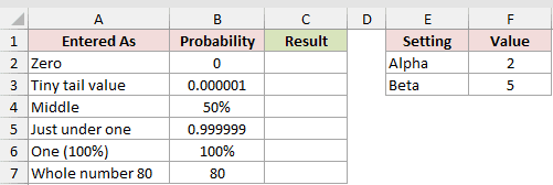
The formula will return a beta value or the expected error for each probability in column C.
Here is the formula entered in C2:
=BETA.INV(B2:B7,$F$2,$F$3)
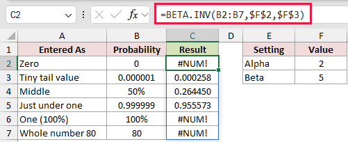
Probabilities of exactly 0 and exactly 1 both return #NUM!. A whole number 80 also returns #NUM! because Excel reads it as 80, not 80%.
The small positive value 0.000001 returns 0.000258, while 0.999999 returns 0.955573.
A probability just inside 0 or 1 returns a usable value close to the bound. Exactly 0 or 1 returns #NUM!.
The 50% row returns 0.264450, matching the same middle percentile shown earlier with alpha 2 and beta 5.
Tips & Common Mistakes
- Keep probability strictly between 0 and 1. Both endpoints return #NUM!, so use a small positive tail probability when that fits your analysis.
- Alpha and beta must both be greater than zero. Excel returns #NUM! when either shape parameter is zero or negative.
- A must be smaller than B. If you provide only A, B still defaults to 1, so an A value above 1 returns #NUM!.
- Non-numeric text returns #VALUE!, while numeric text such as
"0.5"is coerced to a number. - BETA.INV reverses the cumulative BETA.DIST calculation. For example,
BETA.DIST(BETA.INV(0.9,2,5),2,5,TRUE)returns 0.9. - Use PERCENTILE.INC for percentiles from observed data. Use BETA.INV when your percentiles come from a beta distribution model.
- If a range formula returns one value unexpectedly, remove an implicit-intersection
@. In Excel 2019 and earlier, use fill-down formulas or a legacy array formula. - Random formulas are volatile. Copy the results and paste values when you need to preserve one simulation run.
BETA.INV turns a modeled cumulative probability into a bounded value you can use as a threshold, duration, rate, or simulation input.
Its optional bounds keep results in practical units, while alpha and beta control the distribution’s shape.
Related Excel Functions / Articles:
