
Excel’s CHISQ.DIST function returns either the left-tail probability or the probability density for a chi-square value and its degrees of freedom.
The TRUE mode measures the area to the left. The FALSE mode returns the curve’s height, not the probability of observing one exact value.
In this article, I’ll show you how to compare left-tail probabilities, build a distribution table, and test process variation.
CHISQ.DIST Function Syntax in Excel
The CHISQ.DIST function uses a chi-square value, degrees of freedom, and a required cumulative setting.
=CHISQ.DIST(x, deg_freedom, cumulative)
- x (required) is the chi-square value at which you want to evaluate the distribution.
- deg_freedom (required) is the number of degrees of freedom for the distribution.
- cumulative (required) determines the result. TRUE returns the left-tail cumulative probability, while FALSE returns the probability density.
When to Use CHISQ.DIST Function
- Find the probability to the left of a known chi-square statistic.
- Compare the meaning of the same statistic under different degrees of freedom.
- Create density and cumulative values for a chi-square curve.
- Run lower-tail or two-tailed tests of process variation.
- Estimate how often a healthy process will pass a variability check.
Example 1: Find Left-Tail Probabilities
Let’s start by evaluating several production-line checks at once.
Below is the dataset. It lists each filling line, its chi-square statistic, degrees of freedom, and an empty result column for the left-tail probability.
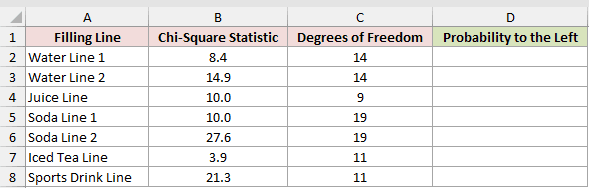
We want one formula to return the probability to the left for every line.
Here is the formula:
=CHISQ.DIST(B2:B8,C2:C8,TRUE)
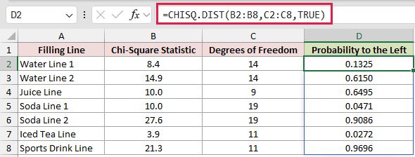
The formula evaluates the statistics in column B against the matching degrees of freedom in column C.
The Juice Line and Soda Line 1 both have a statistic of 10.0. Their probabilities are 0.6495 and 0.0471 because their degrees of freedom differ.
This range formula spills in Excel 2021, Excel 2024, and Microsoft 365. In Excel 2019 and earlier, enter the matching single-row version and fill it down.
Example 2: Compare Density and Cumulative Results
Now let’s put both CHISQ.DIST modes beside the same chi-square values.
Below is the dataset. Column A holds the chi-square values, E2 holds the degrees-of-freedom input, and columns B and C will hold the two results.
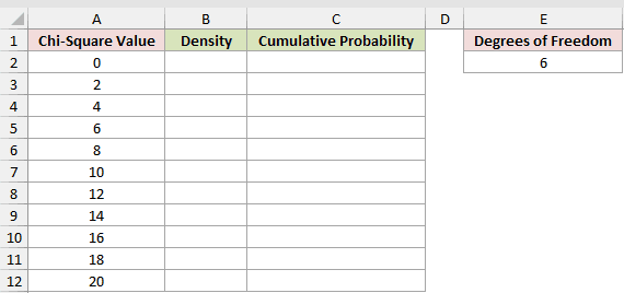
We first want the density at each chi-square value.
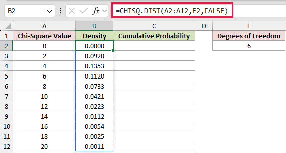
Here is the density formula:
=CHISQ.DIST(A2:A12,E2,FALSE)
Next, we want the cumulative probability for the same values.
Here is the cumulative formula:
=CHISQ.DIST(A2:A12,E2,TRUE)
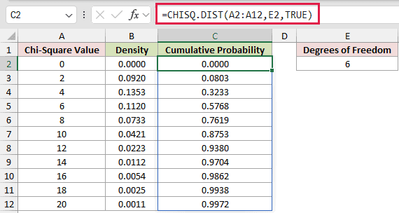
With 6 degrees of freedom, the density reaches 0.1353 at x = 4. That is the curve’s peak, not a probability assigned to exactly 4.
At x = 6, the cumulative result is 0.5768. This is the area of the distribution at or below that value.
Changing E2 redraws both columns for a different distribution, so the table is ready to use as the source for a chart.
Example 3: Test for Lower Process Variation
Here’s a practical lower-tail variance test using measured fill volumes.
Below is the dataset. It contains can IDs, fill volumes, a typed target standard deviation, and labelled cells for the variance, degrees of freedom, statistic, and probability.
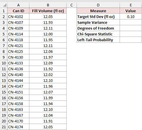
We first need the sample variance of the fill measurements.
Here is the formula:
=VAR.S(B2:B21)
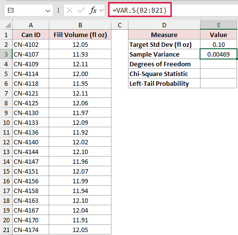
The sample variance in E3 is 0.00469.
Next, we need the degrees of freedom.
Here is the formula:
=COUNT(B2:B21)-1
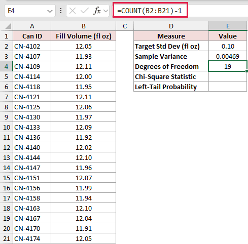
The count calculation returns 19 degrees of freedom in E4.
Now we can calculate the chi-square statistic from the sample variance and the target variance.
Here is the formula:
=E4*E3/E2^2
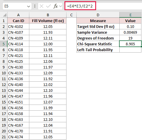
E5 now shows a chi-square statistic of 8.905.
Finally, we can find the probability to the left of that statistic.
Here is the formula:
=CHISQ.DIST(E5,E4,TRUE)
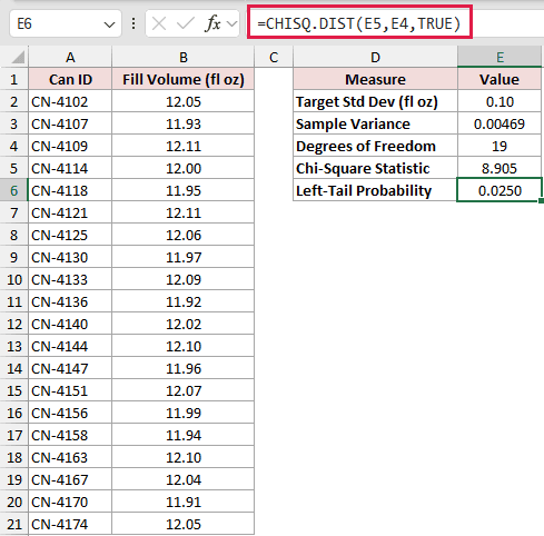
The left-tail probability is 0.0250. A result this small indicates the new filler varies less than the target standard deviation of 0.10 fl oz.
This is a lower-tail question because the test asks whether the process has become more consistent, not whether its variation changed in either direction.
Example 4: Run a Two-Tailed Variance Test
Next, let’s test whether battery runtime consistency changed in either direction.
Below is the parameter card. It holds the battery count, current and old standard deviations, plus labelled cells for the statistic, left-tail comparison, and two-tailed result.
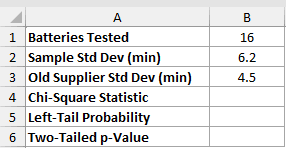
We first want the chi-square statistic for the current sample.
Here is the formula:
=(B1-1)*B2^2/B3^2
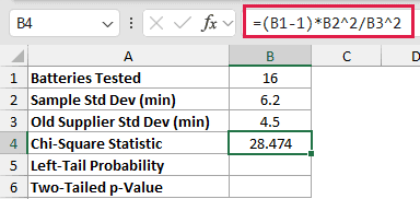
The calculation puts the chi-square statistic, 28.474, in B4.
B5 is the left-tail step used by the two-tailed formula.
Here is the left-tail formula:
=CHISQ.DIST(B4,B1-1,TRUE)
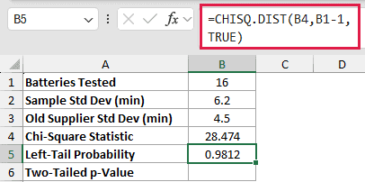
The left tail alone is 0.9812, not the answer for a change in either direction.
For the two-tailed test, we double whichever tail is smaller.
Here is the formula:
=2*MIN(B5,1-B5)
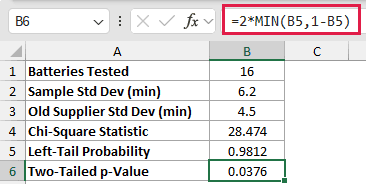
The two-tailed p-value is 0.0376. That is the result to use when either lower or higher variation would count as a change.
For this statistic, CHISQ.DIST.RT(B4,B1-1) returns 0.0188 for the upper tail. Doubling it gives B6’s 0.0376.
Example 5: Estimate a Process Pass Rate
Now let’s use the distribution to plan a bottle-filler check.
Below is the dataset. It lists candidate standard-deviation limits, a result column for pass chances, and typed inputs for bottles per check and healthy process variation.
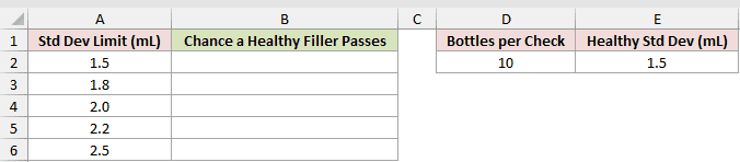
We want the chance that a healthy filler stays within each proposed standard-deviation limit.
Here is the formula:
=CHISQ.DIST((D2-1)*A2:A6^2/E2^2,D2-1,TRUE)
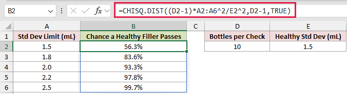
The formula converts each limit into a chi-square value, then returns the probability that a healthy process falls at or below it.
A 1.5 mL limit passes 56.3% of healthy checks. Raising the limit to 2.5 mL increases the pass chance to 99.7%.
The false-alarm rate is one minus the pass chance. If you need a limit for a chosen pass rate, CHISQ.INV answers that reverse question.
Example 6: Flag a Suspiciously Good Fit
Finally, let’s check counts that look almost too evenly distributed.
Below is the dataset. It lists random pulls by filler head and labelled result cells for expected pulls, the statistic, degrees of freedom, and left-tail probability.
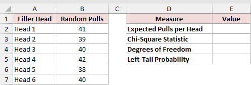
We first need the expected number of pulls for each filler head.
Here is the formula:
=SUM(B2:B7)/ROWS(B2:B7)
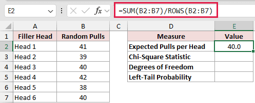
E2 shows 40.0 expected pulls per head.
Next, we calculate how far the observed counts sit from that expectation.
Here is the chi-square statistic formula:
=SUM((B2:B7-E2)^2/E2)
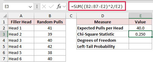
This SUM formula needs Excel 2021, Excel 2024, or Microsoft 365. In Excel 2019 and earlier, press Ctrl+Shift+Enter or use =SUMPRODUCT((B2:B7-E2)^2/E2).
That calculation places 0.250 in E3.
Now we calculate the degrees of freedom from the number of filler heads.
Here is the formula:
=ROWS(B2:B7)-1
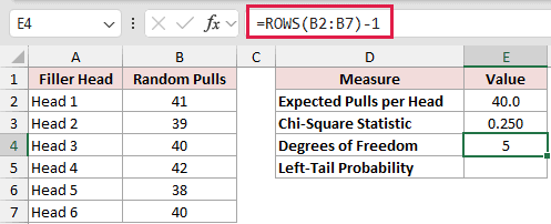
The formula returns 5 degrees of freedom in E4.
Finally, we evaluate the left tail of that statistic.
Here is the formula:
=CHISQ.DIST(E3,E4,TRUE)
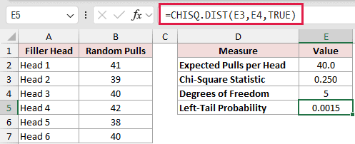
The left-tail probability is 0.0015. That tiny value says the observed counts hug the equal expectation unusually closely for a random process.
A high right-tail result can look reassuring here, but it answers the opposite question. The small left tail is what exposes the overly neat pattern.
Tips & Common Mistakes
- The
cumulativeargument is required. TRUE returns the left-tail cumulative probability, while FALSE returns density. - A blank cell used for
cumulativeacts like FALSE. This silent switch can produce a plausible density when you expected a probability. - Legacy CHIDIST is right-tailed. At x = 3 with 4 degrees of freedom, CHIDIST returns 0.557825 while CHISQ.DIST with TRUE returns 0.442175.
- Negative x values and degrees of freedom below 1 return #NUM!. Excel truncates fractional degrees of freedom, so 1.9 behaves like 1.
- At x = 0, density returns #NUM! with 1 degree of freedom, 0.5 with 2 degrees, and 0 above that.
- Text numbers such as
"3"are converted, while other text returns #VALUE!. - CHISQ.DIST has been available since Excel 2010.
- Use CHISQ.DIST.RT when you need the right tail directly. Replacing CHIDIST with CHISQ.DIST changes the tail and can reverse the interpretation.
Choose the tail before you build the test.
That one decision keeps a plausible density or opposite-tail probability from steering you wrong.
Related Excel Functions / Articles:
