Excel Drop-Down List Not Working – How to Fix?

If your Excel drop-down arrow is missing, the list won’t open, or the items look wrong, start with the symptom you’re seeing.

The arrow only appears when you select a cell with a drop-down. That’s normal. If it still doesn’t appear, check the settings below.

These steps use Excel for Windows (Microsoft 365); on a Mac, use Cmd instead of Ctrl and find the options under Excel > Preferences.

Reason #1: In-Cell Dropdown Is Turned Off

A cell can have a valid list rule without showing a drop-down arrow. This is the first setting I’d check when selecting the cell doesn’t reveal one.

Below I have a dataset of class signups in A1:C9, with Signup ID, Member, and Class headers. The selected Class cell has no arrow.

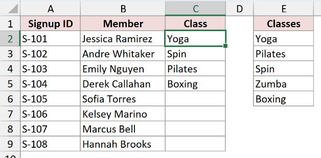
The class choices are Yoga, Pilates, Spin, Zumba, and Boxing in E2:E6, under the Classes header in E1.

C2:C9 already has List validation pointing to that range. However, In-cell dropdown is unchecked, which hides the arrow without removing the rule.

Here are the steps to restore it:

1. Select C2:C9, then go to Data tab > Data Validation > Settings tab. Check In-cell dropdown. Leave Allow set to List and the existing Source unchanged.

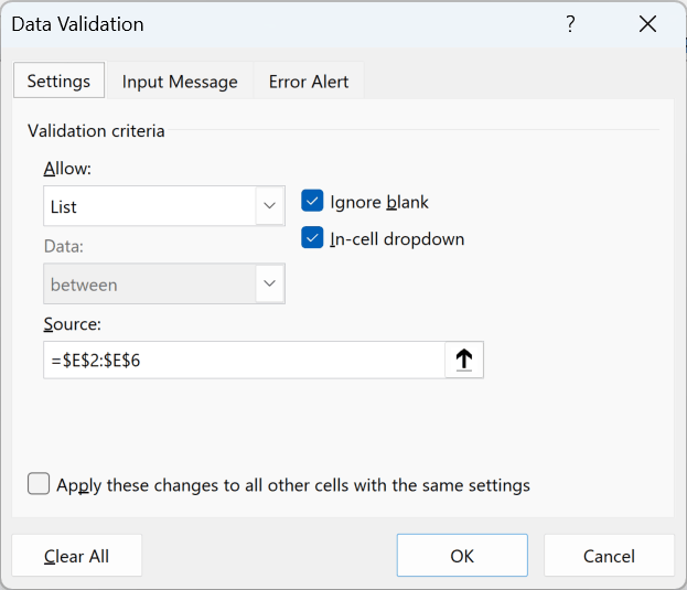
The Source should read:

=$E$2:$E$6

2. Click OK, then select C2 and click its drop-down arrow.

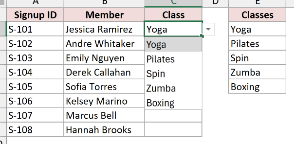
The arrow now opens the five-class list. Other cells in C2:C9 show their arrow when selected.

Reason #2: Workbook Objects Are Hidden

If In-cell dropdown is already checked, look at the workbook’s object display setting next.

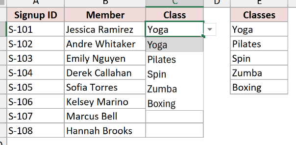
Below I have a dataset of class signups in A1:C9 and a Classes list in E2:E6. With objects hidden, the selected Class cell shows no arrow.

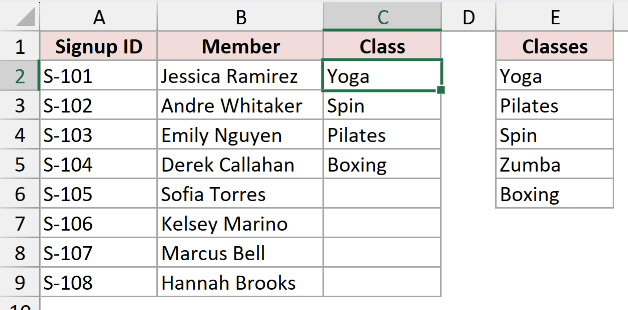
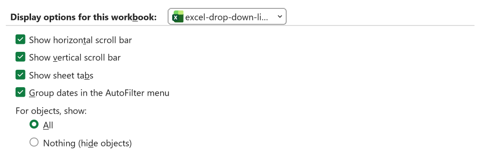
The Reason 2 sheet in the example workbook starts with a working drop-down. The problem appears when For objects, show: is set to Nothing (hide objects).

This setting applies to the workbook, so it can hide drop-down arrows on every sheet in that workbook.

Here are the steps to show them again:

1. Go to File > Options > Advanced. Scroll to Display options for this workbook, check that the affected workbook is selected, and set For objects, show: to All.

2. Click OK, then select C2 and open its drop-down.

The class list opens again without any change to its source or validation rule.

Note: Ctrl+6 toggles objects on and off. It’s easy to press accidentally, so check this workbook setting if several arrows disappear together.

Reason #3: New Items Are Outside the Source Range

A newly added class can be missing from a working drop-down because it falls outside the source range.

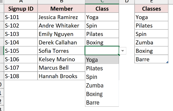
Below I have a dataset of class signups with Barre added in E7. The open drop-down still shows only the five classes in E2:E6.

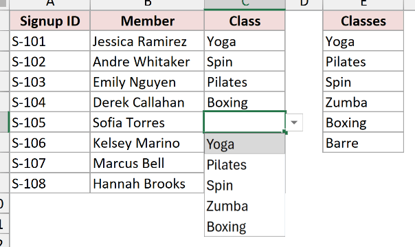
The validation Source still points to:

=$E$2:$E$6

Barre is outside that range. Typing it into E7 doesn’t change the rule’s ending row.

I’ll convert the source to an Excel Table so future additions become available automatically.

Here are the steps:

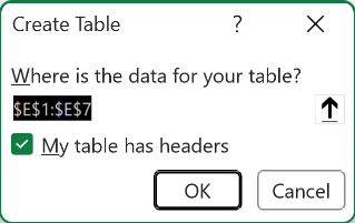
1. Select E1:E7 and press Ctrl+T. Make sure My table has headers is checked, then click OK.

2. With a cell in the table selected, go to Table Design tab > Table Name. Enter ClassList and press Enter.

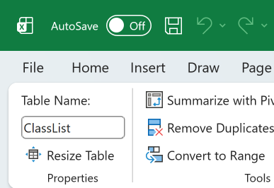
The Source box doesn’t accept a structured reference directly. INDIRECT lets the validation rule use the Classes column in ClassList.

Use this formula as the new Source:

=INDIRECT("ClassList[Classes]")

3. Select C2:C9, go to Data tab > Data Validation > Settings tab, and replace Source with the formula above. Click OK, then open the drop-down in C2.

The list now shows six classes, including Barre. When you type another class directly under the table, the table expands and the drop-down includes it.

Reason #4: The Source Contains Blank Cells

Empty lines between your classes? Look for gaps in the source cells.

Below I have a dataset of class signups with three blank cells in E2:E9. The open Class drop-down shows one empty line between Yoga and Pilates.

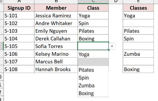
E2:E9 contains Yoga, a blank, Pilates, Spin, a blank, Zumba, a blank, and Boxing. The Source includes that entire range:

=$E$2:$E$9

Those blank source cells become empty entries in the drop-down. The fix is to remove the gaps and shorten the reference.

Here are the steps to clean up the list:

1. Replace the contents of E2:E9 with the five classes in consecutive cells: E2 Yoga, E3 Pilates, E4 Spin, E5 Zumba, and E6 Boxing. Clear the leftover contents in E7:E9.

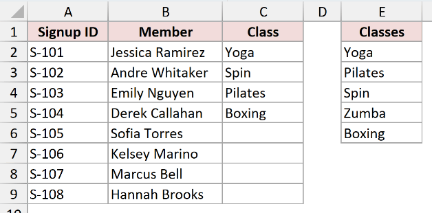
The corrected Source is:

=$E$2:$E$6

2. Select C2:C9 and go to Data tab > Data Validation > Settings tab. Set Source to the reference above, click OK, and open the drop-down in C2.

The list now shows Yoga, Pilates, Spin, Zumba, and Boxing without empty lines between them.

Reason #5: The Source Sheet Was Deleted

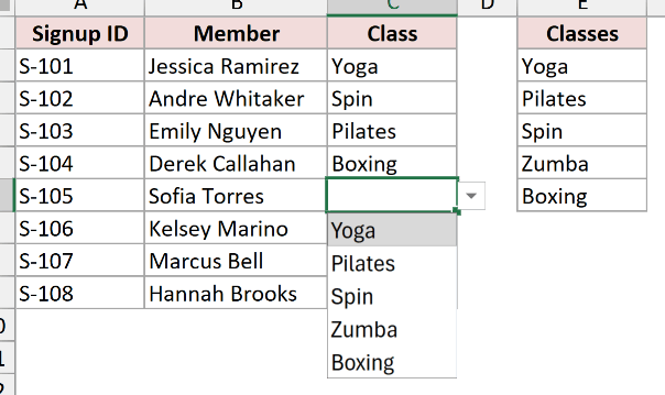
With no items to show, the validation rule may have lost its source.

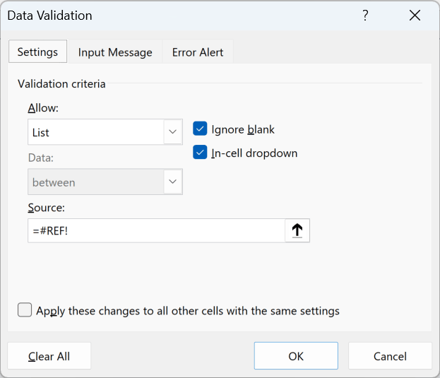
I’ve opened Data Validation’s Settings tab for the Class cells (C2:C9). The Source reads =#REF! because the sheet holding the list was deleted.

Clicking the arrow opens no list at all.

The #REF! means the Source is broken, so the drop-down has no valid items to show.

Here are the steps to rebuild the source:

1. Enter Classes in E1. Fill E2:E6 with Yoga, Pilates, Spin, Zumba, and Boxing, in that order.

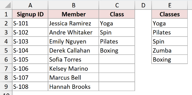
Point the rule to the rebuilt list using this Source:

=$E$2:$E$6

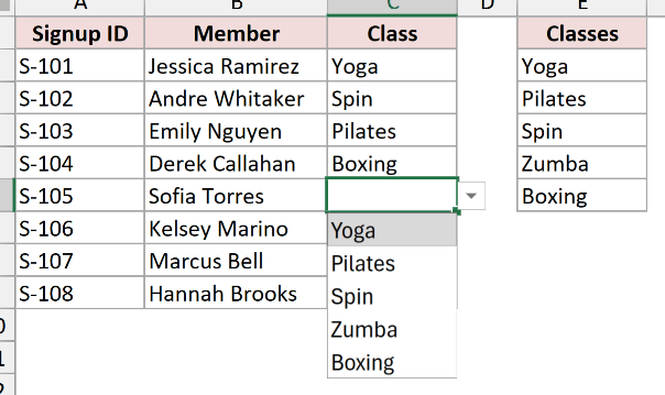
2. Select C2:C9, then go to Data tab > Data Validation > Settings tab. Replace the broken Source with the reference above. Click OK and open the drop-down in C2.

The five classes are available again because the rule points to cells that exist.

Note: For a workbook with several lists, keep the sources on a dedicated sheet and don’t delete that sheet while validation rules depend on it.

Reason #6: The Error Alert Is Turned Off

Sometimes the list opens correctly, but Excel accepts a typed value that isn’t one of the choices.

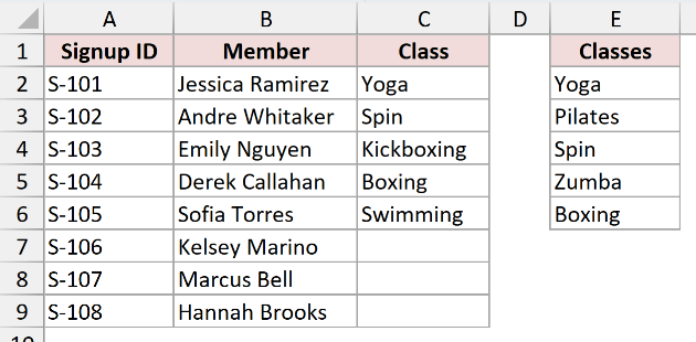
Below I have a dataset of class signups with Kickboxing in C4 and Swimming in C6. Neither value appears in the Classes list in E2:E6.

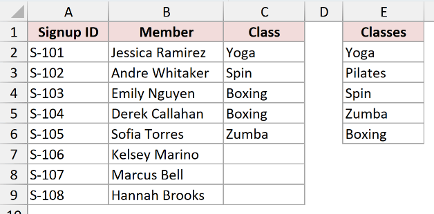
Show error alert after invalid data is entered is unchecked on the Error Alert tab. The drop-down offers choices, but invalid typed entries aren’t blocked.

Turning the alert back on won’t replace incorrect values already stored in the cells. I’ll fix those after restoring the setting.

Here are the steps:

1. Select C2:C9 and go to Data tab > Data Validation > Error Alert tab. Check Show error alert after invalid data is entered, set Style to Stop, and click OK.

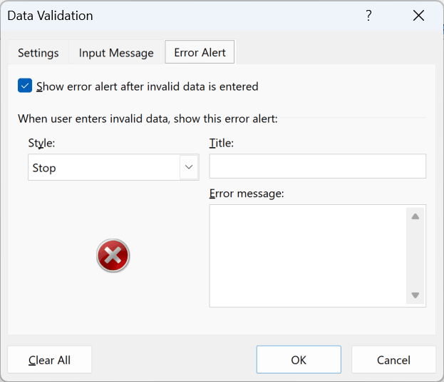
2. Replace Kickboxing in C4 with Boxing and Swimming in C6 with Zumba, using each cell’s drop-down.

C4 now contains Boxing and C6 contains Zumba. The Stop alert blocks invalid values typed into the validated cells.

Note: Warning and Information alerts still let someone keep an invalid entry after clicking through the message. Use Stop when typed entries must match the list.

Reason #7: Pasting Removed the Validation Rule

Missing arrows in just a few cells can mean a paste replaced their validation rules.

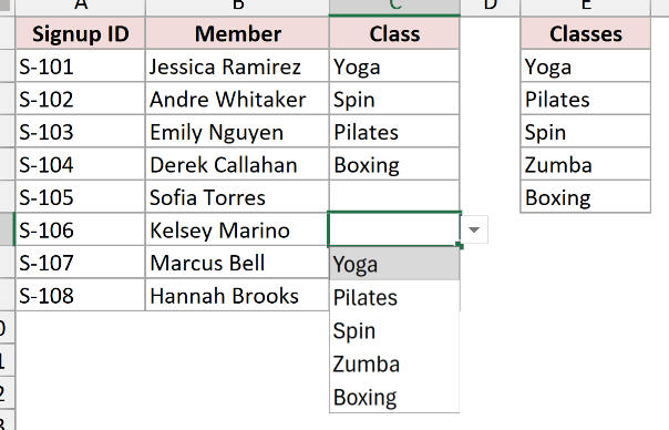
Below I have a dataset of class signups where C2:C6 keeps its drop-downs, but the selected cell in C7:C9 has no arrow.

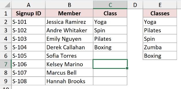
Plain cells were copied and pasted over C7:C9. A full paste can replace the destination’s validation along with its contents.

C2 still has the correct rule, so I’ll copy only its validation to the affected cells.

Here are the steps to restore the missing rules:

1. Copy C2 and select C7:C9. Go to Home > Paste > Paste Special, or press Ctrl+Alt+V. Select Validation.

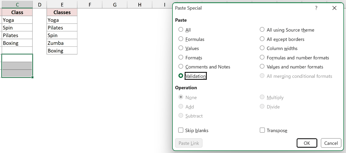
2. Click OK, then select C7 and open its drop-down.

C7:C9 now has the same five-class validation rule as C2. Pasting Validation preserves the destination cells’ existing contents.

Note: Use Paste Values when adding data to a drop-down column to preserve its validation rules. Still check the pasted values, since pasting can bypass validation alerts.

Reason #8: The Protected Sheet Has Locked Cells

A protection message when you choose a class is a clue that the drop-down cells may be locked.

Below I have a dataset of class signups in A1:C9 on a protected sheet. Trying to change a Class entry shows a protection message.

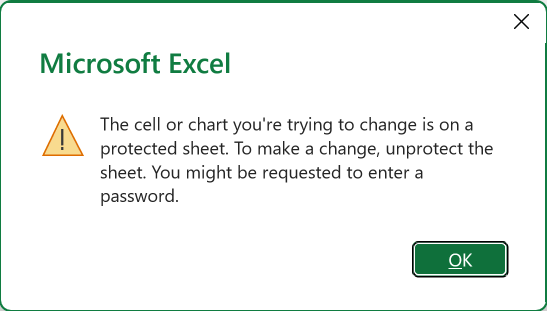
C2:C9 is locked. Once sheet protection is enabled, Excel prevents changes to those cells, including changes made through a drop-down.

I’ll unlock the Class cells and then protect the sheet again.

Here are the steps:

1. Go to Review tab > Unprotect Sheet. Enter the sheet password if prompted.

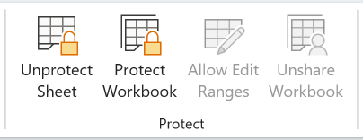
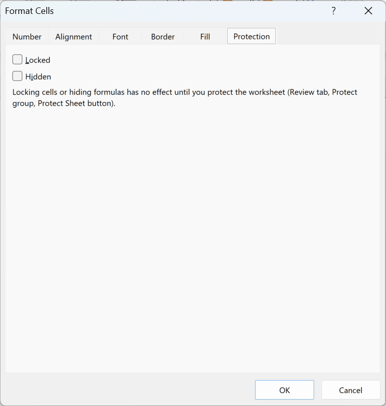
2. Select C2:C9 and press Ctrl+1. On the Protection tab, uncheck Locked and click OK.

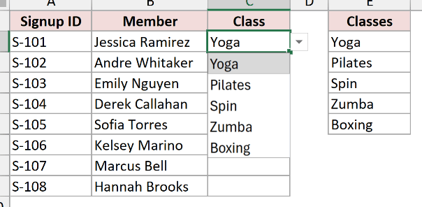
3. Go to Review > Protect Sheet and confirm the protection settings, allowing selection of unlocked cells. Then select C2 and choose Yoga from its drop-down.

The drop-down now works in C2:C9 while the rest of the locked cells stay protected.

Reason #9: Dependent List Names Contain Spaces

For a dependent drop-down that works for some categories but not others, compare the category text with the named ranges.

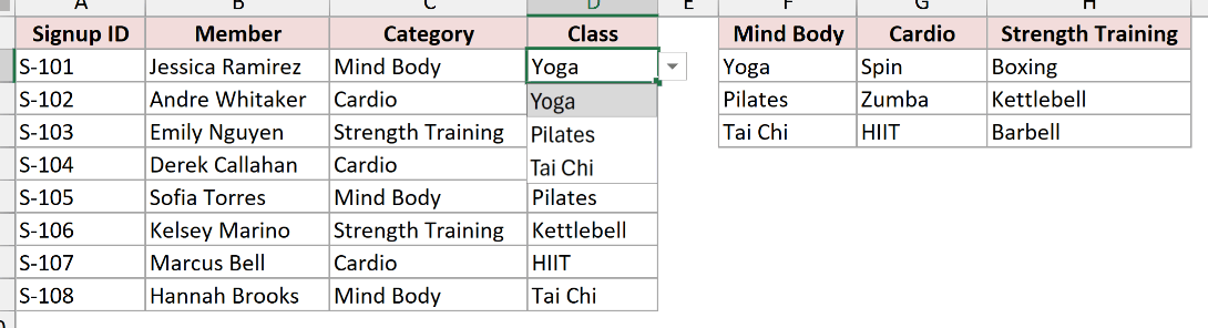
Below I have a dataset in A1:D9 with Signup ID, Member, Category, and Class headers. Cardio rows have class selections, while the other categories’ Class cells are blank.

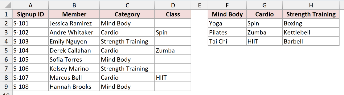
C2:C9 contains Mind Body, Cardio, Strength Training, Cardio, Mind Body, Strength Training, Cardio, and Mind Body.

The source lists sit in columns F:H:

• F1 is Mind Body, with Yoga, Pilates, and Tai Chi below it.
• G1 is Cardio, with Spin, Zumba, and HIIT below it.
• H1 is Strength Training, with Boxing, Kettlebell, and Barbell below it.

The named ranges are Mind_Body, Cardio, and Strength_Training. Excel names can’t contain spaces.

When you create names through Formulas > Create from Selection > Top row, Excel replaces the spaces in those headers with underscores.

However, D2:D9 uses this Source:

=INDIRECT(C2)

For C2, INDIRECT tries to resolve Mind Body, but the actual name is Mind_Body. The same mismatch affects Strength Training.

Cardio has no spaces, so those rows work. D3 contains Spin, D5 contains Zumba, and D8 contains HIIT.

Here is the corrected Source formula:

=INDIRECT(SUBSTITUTE(C2," ","_"))

Here are the steps to apply it:

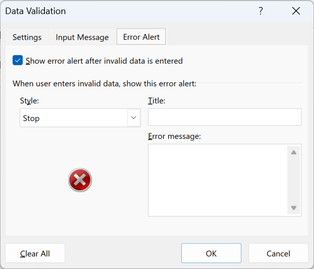
1. Select D2:D9 with D2 as the active cell. Go to Data tab > Data Validation > Settings tab. Replace Source with the corrected formula above and click OK.

How does this formula work?

SUBSTITUTE replaces each space in C2 with an underscore. Mind Body becomes Mind_Body, which matches the existing named range.

INDIRECT turns that text into a reference to the matching class list. Cardio stays Cardio because there’s no space to replace.

C2 is a relative reference, so each validated row uses its own Category cell. Keep it exactly as shown when applying the rule from D2.

2. Use the repaired drop-downs to select Yoga in D2, Boxing in D4, Pilates in D6, Kettlebell in D7, and Tai Chi in D9.

D2:D9 now contains Yoga, Spin, Boxing, Zumba, Pilates, Kettlebell, HIIT, and Tai Chi. Each category opens its matching list.

Frequently Asked Questions

Why Does My Drop-Down Arrow Only Show on One Cell?

Excel displays the data validation arrow only for the selected cell. Moving to another cell hides the previous arrow, even though its validation rule remains.

How Do I Make a Drop-Down List Update Automatically?

Use an Excel Table for the source and point validation to its column through INDIRECT. I’ve shown the setup in Reason #3 above.

Can I Make the Drop-Down List Font Bigger?

The standard data validation list has a fixed font size. Increasing the worksheet zoom is a workaround for making it easier to read.

The list shows eight items at a time, then scrolls to the remaining choices.

Why Can I Type Values That Aren’t in the Drop-Down?

Check that Error Alert is enabled and uses Stop. Warning and Information let you accept an invalid entry after the alert appears.

Ignore blank can also allow invalid entries in some setups where the source contains blank cells.

Conclusion

I’d start by selecting the cell and checking In-cell dropdown in Data Validation. That gives you a simple first check before looking further.

I hope this helped you get your list working again.

Other Excel articles you may also like:

• How to Remove Drop-down List in Excel?
• How to Select Multiple Items from a Drop Down in Excel?