If you want to turn a piece of text like “B3” into a real, working cell reference, the INDIRECT function is what you’re after.
It lets you decide which cell or range a formula points to based on text, so you can change the target without touching the formula itself.
INDIRECT does not spill. It returns one reference per call, so each formula gives you a single result. In this article, I’ll walk you through how it works with five simple examples.
INDIRECT Function Syntax in Excel
Here is the syntax of the INDIRECT function:
=INDIRECT(ref_text, [a1])
- ref_text: The reference written as a text string. This can be a cell address like “B3”, a range like “B2:B5”, or a named range.
- [a1]: Optional. Use TRUE (or leave it out) to read ref_text as a normal A1-style reference. Use FALSE to read it as R1C1 style.
When to Use INDIRECT Function
- When you want to build a cell reference from text that other cells supply, like a column letter plus a row number.
- When you need a formula to keep pointing at the same cells even after rows or columns are inserted.
- When you want to pull data from a sheet whose name is typed in a cell.
- When you are setting up dependent drop-down lists that change based on another cell’s value.
Example 1: Turn a Text String into a Cell Reference
Let’s start with the most basic use of INDIRECT.
Below is the dataset. Column A has product names, column B has the units sold, and cell D2 holds a cell address typed as plain text.
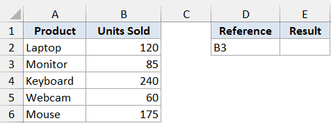
I want to pull whatever value sits in the cell that D2 names. Right now D2 contains “B3”.
Here is the formula:
=INDIRECT(D2)
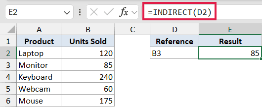
INDIRECT takes the text “B3” from D2 and turns it into a real reference to cell B3. Since B3 holds 85, the units sold for Monitor, the formula returns 85.
Change D2 to “B5” and the result updates to the value in B5. The formula never changes, only the text it reads.
Pro Tip: The text inside INDIRECT must spell out a reference Excel recognizes. A typo like “BB3” or an extra space returns a #REF! error.
Example 2: Build a Reference from a Row Number
Here’s a more flexible scenario.
Below is the dataset. Column A lists employees, column B lists their sales, and cell D2 holds a row number.
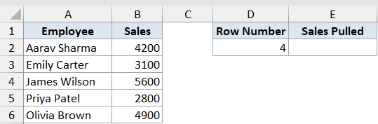
I want to pull the sales figure from whatever row number you put in D2. Right now D2 is 4.
Here is the formula:
=INDIRECT("B"&D2)
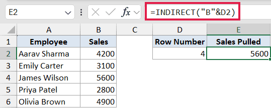
The ampersand joins the column letter “B” with the number in D2, building the text “B4”. INDIRECT turns that into a reference to B4, which holds 5600, James Wilson’s sales.
This is handy when the column stays the same but the row you want changes based on another input.
Example 3: Sum a Range That Is Written as Text
INDIRECT also works nicely inside other functions.
Below is the dataset. Column A has quarters, column B has revenue, and cell D2 holds a range written as text.
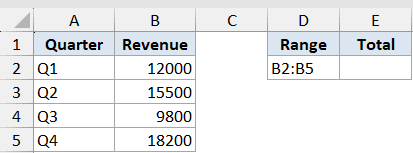
I want to total the revenue for the range named in D2, which contains “B2:B5”.
Here is the formula:
=SUM(INDIRECT(D2))
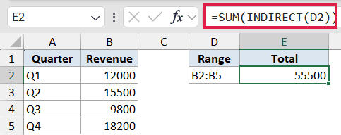
INDIRECT converts the text “B2:B5” into a real range, and SUM adds it up. The four quarters total 55,500.
Because the range lives in a cell, you can point SUM at a different block just by editing D2, without rewriting the formula.
Example 4: Pull a Value by Row and Column Number
You can combine INDIRECT with the ADDRESS function to grab a cell by its position.
Below is the dataset. Columns B to D hold quarterly figures for four regions, and cells F2 and G2 hold a row number and a column number.
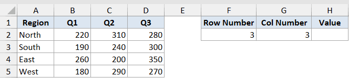
I want the value that sits at the row and column number given in F2 and G2. Here they are both 3.
Here is the formula:
=INDIRECT(ADDRESS(F2,G2))
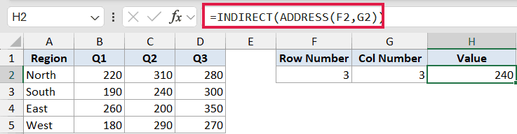
ADDRESS(3,3) builds the text “$C$3”, and INDIRECT turns it into a live reference. Cell C3 holds 240, which is South’s Q2 figure, so that’s what comes back.
This is useful when you already have row and column numbers and want to fetch the cell where they meet.
Example 5: Lock a Reference So It Does Not Shift
This is one of INDIRECT’s most underrated uses.
Below is the dataset. Column A lists months and column B lists the expenses for six months.
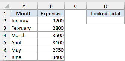
I want a total that always points at cells B2 to B7, even if someone inserts a new row inside that range.
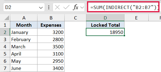
Here is the formula:
=SUM(INDIRECT("B2:B7"))
A normal =SUM(B2:B7) adjusts itself when you insert rows. Add a row inside it and Excel quietly rewrites it to =SUM(B2:B8).
INDIRECT works differently. Because “B2:B7” is just text, it always points at those exact cells, no matter what you insert or delete. That makes it a simple way to anchor a reference in place.
Pro Tip: INDIRECT is a volatile function, which means it recalculates every time the workbook changes. A handful is fine, but hundreds of them can slow a large file down.
Tips & Common Mistakes
- A #REF! error almost always means the text doesn’t resolve to a valid reference. Check for typos, stray spaces, or a sheet name that no longer exists.
- INDIRECT can’t read a closed workbook. References to another file only work while that file is open, otherwise you get a #REF! error.
- To pull a value from another sheet named in a cell, build the reference like =INDIRECT(“‘”&A1&”‘!B2”), where A1 holds the sheet name. It’s a common way to roll up data from many sheets.
- Excel’s formula auditing tools can’t trace through INDIRECT, since the reference is just text. Keep a note of what it points to so it’s easy to follow later.
- In Excel 365, the old ROW(INDIRECT(“1:10”)) trick for building a list of numbers is no longer needed. Use SEQUENCE(10) instead.
INDIRECT is one of those functions that looks small but opens up a lot of flexible options. Once you get comfortable building references from text, you can make your formulas adjust to whatever your sheet throws at them.
Try it out with the examples above and see where it fits into your own work.
Related Excel Functions / Articles: