
Excel’s ERROR.TYPE function returns a number identifying an error in a cell. Division by zero returns code 2, while a missing lookup result returns code 7.
These codes let you show different messages for different problems. A cell without an error makes ERROR.TYPE return #N/A, so successful calculations need handling too.
ERROR.TYPE Function Syntax in Excel
ERROR.TYPE takes one required argument:
=ERROR.TYPE(error_val)
- error_val: The error value, formula, or cell reference you want to identify. A range can return multiple codes in Excel versions that support dynamic arrays.
When to Use ERROR.TYPE Function
- Identify which error a formula returned.
- Display a specific message for each kind of error.
- Replace one error type while keeping other errors visible for investigation.
- Count errors by type to prioritize corrections in a worksheet.
Example 1: Identify Excel Error Codes
Let’s start by checking several formula results together.
Below is the dataset with descriptions in column A, existing formula results in column B, and empty cells under Error Code in column C.
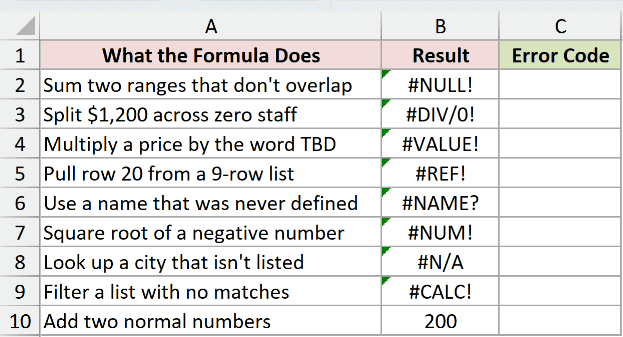
We want to identify the errors in B2:B10 by entering one formula in C2.
Here is the formula:
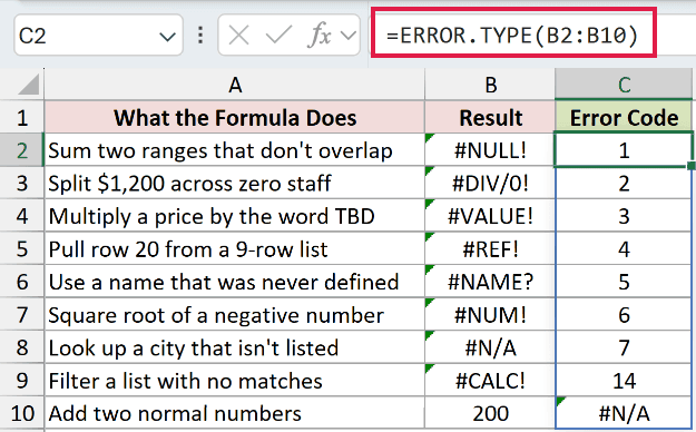
=ERROR.TYPE(B2:B10)
How this formula works:
ERROR.TYPE checks each cell in B2:B10 and returns its result in the corresponding row of C2:C10.
The first seven rows demonstrate these codes:
#NULL!returns 1. The ranges in the first calculation don’t overlap.#DIV/0!returns 2. The calculation tries to split $1,200 across zero staff.#VALUE!returns 3. Multiplying the text “TBD” by a price cannot produce a numeric result.#REF!returns 4. The calculation requests row 20 from a nine-row range.#NAME?returns 5. The formula uses the undefined name TaxRate.#NUM!returns 6. The formula requests the square root of a negative number.#N/Areturns 7. The lookup cannot find Denver in its list of cities.
In row 9, FILTER finds no matches for “Refund” in A2:A10, so B9 returns #CALC!. In Microsoft 365 testing, ERROR.TYPE returned 14 in C9.
That code is an observed result. Microsoft’s documented list stops at 8 and does not include #CALC!.
B10 contains the valid result 200, so C10 returns #N/A. Compare that with B8: an actual #N/A input returns the number 7 in C8.
ERROR.TYPE’s own #N/A result tells you the input wasn’t an error.
Pro Tip: Excel 2021, Excel 2024, and Microsoft 365 support this spill and row 9’s FILTER. Older versions need single-cell checks filled down. Leave C3:C10 empty.
Example 2: Show a Message for Each Error
Let’s label the errors in a fitness class revenue report so you can see which inputs need checking.
Below is the dataset with fitness classes, revenue, attendees, existing Revenue per Attendee calculations, and an empty Issue column.
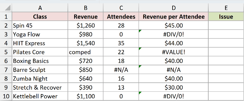
We want E2:E10 to explain each error in D2:D10 and show “OK” for valid calculations.
Here is the formula:
=IFNA(SWITCH(ERROR.TYPE(D2:D10),2,"No attendees",3,"Revenue not a number",7,"Attendance missing","Other error"),"OK")
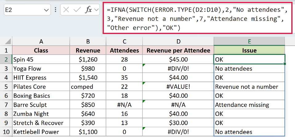
Enter the formula in E2. It fills the Issue column automatically.
How this formula works:
ERROR.TYPE(D2:D10)returns an error code for each failed calculation and#N/Afor each valid result.SWITCHmaps code 2 to “No attendees”, code 3 to “Revenue not a number”, and code 7 to “Attendance missing”.- The final SWITCH argument, “Other error”, handles error codes without a listed message.
IFNAchanges the#N/Aproduced for valid calculations to “OK”.
Yoga Flow has revenue of $980 but zero attendees. Its division error becomes “No attendees”. Kettlebell Power receives the same message.
Pilates Core has “comped” in Revenue, so its issue becomes “Revenue not a number”. Barre Sculpt’s missing attendance produces “Attendance missing”.
Spin 45 returns $45.00 per attendee and receives “OK”.
The original #N/A for Barre Sculpt becomes code 7 before IFNA runs. That lets the formula distinguish missing attendance from a successful calculation.
Pro Tip: Check both inputs before labeling code 3 as revenue text. SWITCH requires Excel 2019 or later; older formulas can map sequential codes with CHOOSE.
Example 3: Replace Only Division Errors
Sometimes you want to handle an expected error while keeping unexpected problems visible.
Below is the dataset with sales reps, leads, deals closed, existing Close Rate calculations, and empty Rate for Report cells.
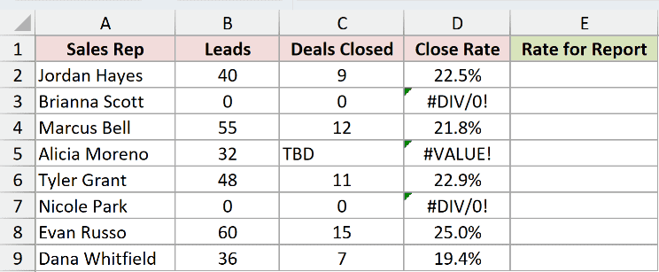
For this report, we want zero leads to display as 0.0%, while other errors remain visible in E2:E9.
Here is the formula:
=IF(IFNA(ERROR.TYPE(D2:D9),0)=2,0,D2:D9)
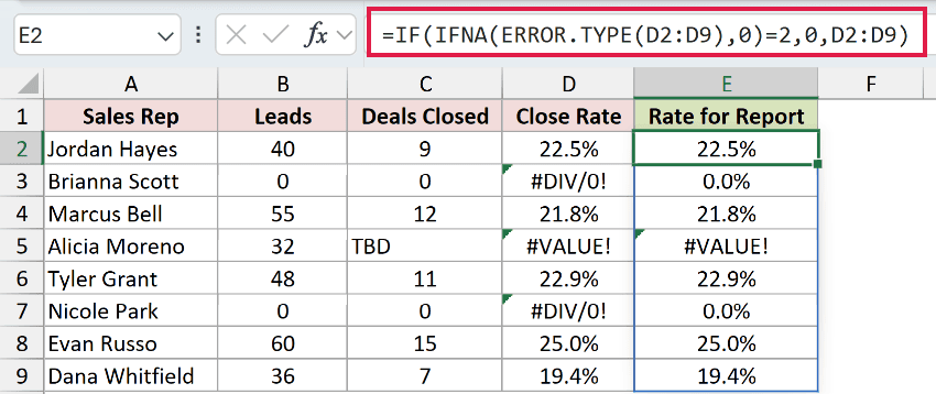
Enter the formula in E2 to fill the report column.
How this formula works:
ERROR.TYPE(D2:D9)identifies the errors in the existing close rates.IFNA(...,0)assigns 0 to valid inputs for the error-code test. It does not replace the original close rates.- The comparison checks whether each code equals 2, the code for
#DIV/0!. IFreturns 0 for those division errors. Otherwise, it returns the original value from D2:D9, including any other error.
Brianna Scott and Nicole Park both have zero leads. Their #DIV/0! results become 0.0% in the report column.
Alicia Moreno has “TBD” under Deals Closed. Her #VALUE! remains visible in E5, so someone can correct the input.
Jordan Hayes keeps the original 22.5% close rate, and Evan Russo keeps 25.0%.
Pro Tip: Use 0.0% for zero leads only if your report allows that convention. Replacing every error with IFERROR would also hide Alicia’s invalid input.
Example 4: Count Errors by Type
You can also use the codes to build a small error summary.
Below is the dataset with SKU costs, existing Cost per Unit results, a units lookup, and an error summary with empty Count cells.
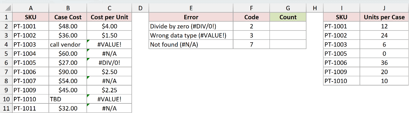
We want G2:G4 to count the errors in C2:C11 that match the codes in F2:F4.
Here is the formula:
=SUMPRODUCT(--(IFNA(ERROR.TYPE($C$2:$C$11),0)=F2))
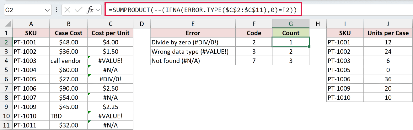
Enter the formula in G2, then fill it down to G4. Each summary row returns one count.
How this formula works:
ERROR.TYPE($C$2:$C$11)identifies each error in Cost per Unit.IFNA(...,0)turns the results for valid costs into 0, leaving actual error codes intact.=F2checks each code against the summary row’s code. In the first row, that code is 2.- The double negative converts TRUE and FALSE to 1 and 0. SUMPRODUCT adds those numbers to count matching errors.
- The dollar signs keep C2:C11 fixed when you fill down. The relative reference F2 changes to F3 and F4.
The summary returns 1 division error, 2 value errors, and 3 missing lookup errors.
PT-1005 has zero units per case, causing the division error. The text costs “call vendor” and “TBD” cause the two value errors.
PT-1004, PT-1007, and PT-1011 are missing from the units lookup, so their costs per unit return #N/A.
Tips & Common Mistakes
- A valid input returns
#N/A, not 0. Wrap the classification in IFNA when you need a usable value for comparisons or summaries. - An actual
#N/Ainput returns 7. This differs from the#N/AERROR.TYPE produces when its input is valid. - Use the function that matches your question. ISERROR checks for any error, ISERR excludes
#N/A, and ISNA checks only#N/A. ERROR.TYPE identifies which error occurred. - Choose replacements deliberately. IFERROR replaces any error; IFNA replaces only
#N/A. ERROR.TYPE lets you build handling around another specific error code. - Don’t treat the classic code list as exhaustive. Microsoft documents codes 1 to 8, including
#GETTING_DATAas 8. In Example 1, Microsoft 365 returned the undocumented code 14 for#CALC!. Verify other newer errors before assigning messages to their codes. - Leave room for spilled results. Occupied output cells can cause
#SPILL!. Examples 1 to 3 use dynamic arrays; Example 4 returns one count per summary row.
Keep the original error cells beside your messages so you can check the formulas when fixing an input.
Related Excel Functions / Articles:
