
The FISHER function in Excel converts a correlation coefficient into Fisher’s z, a transformed value used to compare correlations.
Correlations sit on a bounded scale. FISHER stretches that scale, especially near its ends, so you can do statistical calculations before converting back with FISHERINV.
In this article, I’ll show you how to transform correlations, build confidence intervals, and average correlations without using the raw values directly.
FISHER Function Syntax in Excel
FISHER takes the correlation you want to transform:
=FISHER(x)
- x (required): A number or cell reference containing the correlation coefficient. It must be greater than -1 and less than 1.
FISHER returns the correlation on the Fisher z scale. The examples below add the sample size and normal-distribution functions when a statistical test is needed.
When to Use FISHER Function
- Convert a column of correlations to the Fisher z scale.
- Test whether a correlation differs from zero using an approximate normal test.
- Calculate confidence limits for a correlation, then convert those limits back with FISHERINV.
- Compare correlations from independent groups.
- Combine correlations across seasons or plan the sample size for a correlation study.
Example 1: Transform a Column of Correlations
Let’s start with basketball statistics and their correlations with wins.
Below is the dataset. Column A lists team statistics, column B contains their correlations with wins, and column C is reserved for Fisher z.
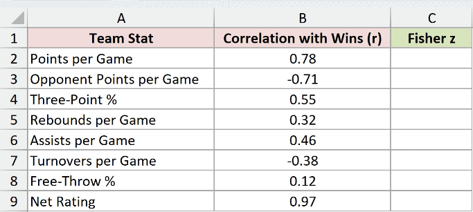
We want to transform each correlation while keeping it beside its original statistic.
Enter this formula in C2:
=FISHER(B2:B9)
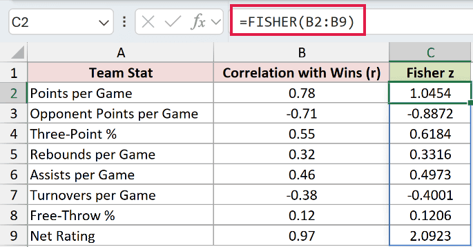
The results spill into C2:C9 in Excel 2021, Excel 2024, and Microsoft 365. In Excel 2019 and earlier, reference each row’s correlation and fill down.
Free-Throw % barely changes: its correlation of 0.12 becomes 0.1206. Net Rating stretches much more, from 0.97 to 2.0923.
The sign stays intact. Opponent Points per Game has a correlation of -0.71 and returns -0.8872.
The transformed scale allows Fisher z values above 1, as the Net Rating result shows.
Example 2: Test Whether a Correlation Is Significant
The same correlation can tell a different story when the sample sizes differ.
Below is the dataset. Columns A:C contain retail metric pairs, correlations, and weeks observed. Columns D:E will hold the test statistic and p-value.
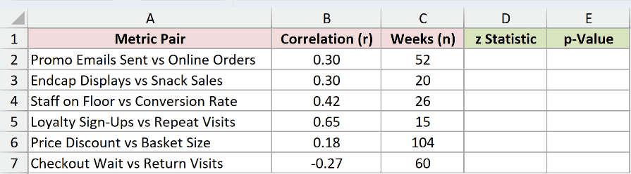
We want an approximate two-tailed test of whether each population correlation differs from zero.
Enter the test-statistic formula in D2:
=FISHER(B2:B7)*SQRT(C2:C7-3)
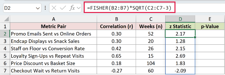
FISHER transforms each correlation. Multiplying by SQRT(n-3) is the same as dividing by the standard error, 1/SQRT(n-3), where n is the sample size.
Promo Emails Sent vs Online Orders returns 2.17. Endcap Displays vs Snack Sales returns 1.28, despite both correlations being 0.30.
Now enter the p-value formula in E2:
=2*(1-NORM.S.DIST(ABS(D2:D7),TRUE))
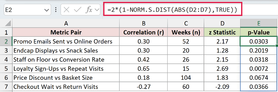
ABS makes the test work in either direction. NORM.S.DIST supplies the cumulative normal probability, and the remaining arithmetic includes both tails.
The email relationship, observed over 52 weeks, returns 0.0303. The endcap relationship, observed over 20 weeks, returns 0.2019.
At a 5% significance level, the email result is significant; the endcap result isn’t.
Pro Tip: This is a Fisher z approximation. For a small-sample test against zero, the t-test route using T.DIST.2T is the usual exact approach under the normal-model assumptions. Statistical significance doesn’t establish causation.
Example 3: Calculate Correlation Confidence Intervals
An interval shows the uncertainty that a correlation alone leaves out.
Below is the dataset. Each department has a correlation and response count, with columns for both limits. The confidence-level input is in H2.
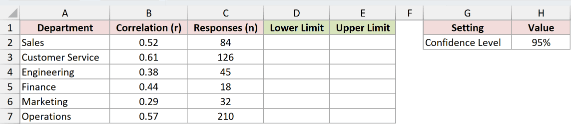
We want confidence intervals for the relationship between manager-support scores and employee-engagement scores.
H2 is a typed input, currently 95%. Enter the lower-limit formula in D2:
=FISHERINV(FISHER(B2:B7)-NORM.S.INV(1-(1-$H$2)/2)/SQRT(C2:C7-3))
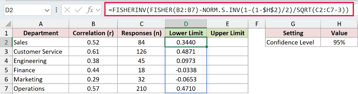
The formula transforms each correlation, subtracts a margin on the z scale, and uses FISHERINV to return the lower limit on the correlation scale.
Sales has a lower limit of 0.3440. Finance has a lower limit of -0.0338.
Enter the upper-limit formula in E2:
=FISHERINV(FISHER(B2:B7)+NORM.S.INV(1-(1-$H$2)/2)/SQRT(C2:C7-3))
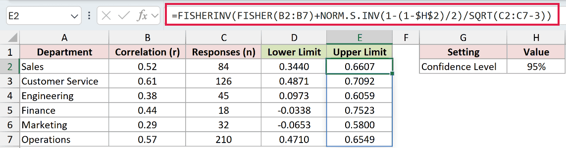
This adds the margin before converting back. Both formulas spill, and the absolute reference $H$2 keeps every department on the same confidence level.
The confidence level determines the critical value used in the margin.
- NORM.S.INV finds the critical normal value for the confidence level, splitting the remaining probability across both tails.
- The standard error is the reciprocal of the square root of the response count minus 3.
- FISHERINV converts the completed limits back to correlations.
Sales returns a 95% confidence interval from 0.3440 to 0.6607 around its correlation of 0.52. The distances on either side aren’t equal.
Finance runs from -0.0338 to 0.7523, and Marketing from -0.0653 to 0.5800. Both intervals include zero, despite their positive sample correlations.
Pro Tip: Don’t add a symmetric margin directly to the raw correlation. Build the interval on the Fisher z scale, then back-transform. CONFIDENCE.NORM and CONFIDENCE.T calculate margins for means, not correlations.
Example 4: Compare Correlations Between Survey Groups
Now let’s check whether a lower survey correlation represents a statistically significant change.
Below is the dataset. B1:B4 contain each year’s correlation and response count. The labeled cells below them hold transformations, standard error, test statistic, and p-value.
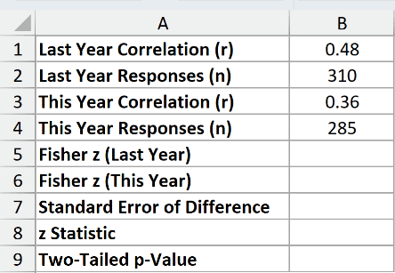
We want to compare the relationship between recognition for good work and intent to stay across independent annual survey groups.
This comparison assumes independent samples. It isn’t the appropriate test when the same employees supply paired responses across years.
Transform last year’s correlation in B5:
=FISHER(B1)
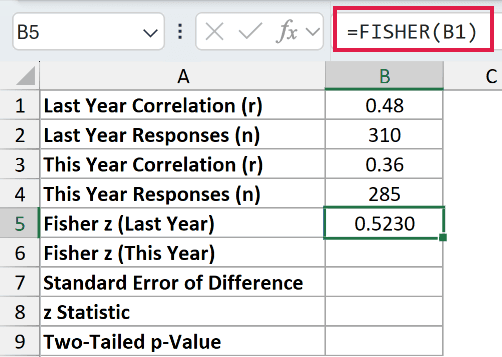
The correlation of 0.48 becomes 0.5230.
Transform this year’s correlation in B6:
=FISHER(B3)
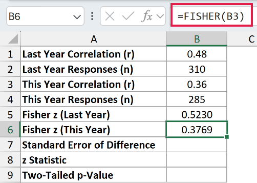
The correlation of 0.36 becomes 0.3769.
Calculate the standard error of the difference in B7:
=SQRT(1/(B2-3)+1/(B4-3))
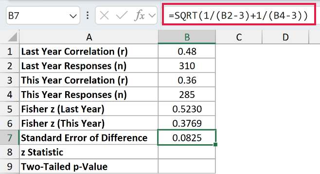
Using the response counts of 310 and 285, this returns 0.0825.
Calculate the test statistic in B8:
=(B5-B6)/B7
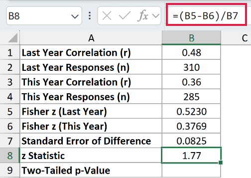
The difference between the transformed correlations, divided by its standard error, returns 1.77.
Finish with the two-tailed p-value in B9:
=2*(1-NORM.S.DIST(ABS(B8),TRUE))
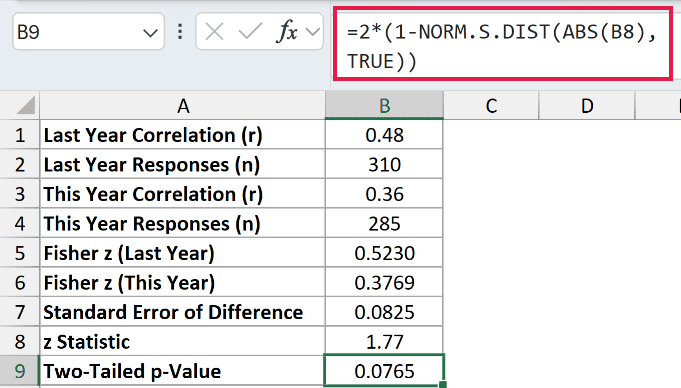
The p-value is 0.0765. At a 5% significance level, the observed drop isn’t statistically significant. That doesn’t prove the population correlations are identical.
Example 5: Average Correlations Across Seasons
Let’s combine one soccer club’s seasonal correlations into an overall estimate.
Below is the dataset. Columns A:C list soccer seasons, correlations, and match counts. The approach labels in E2:E4 identify the calculations shown in column F.
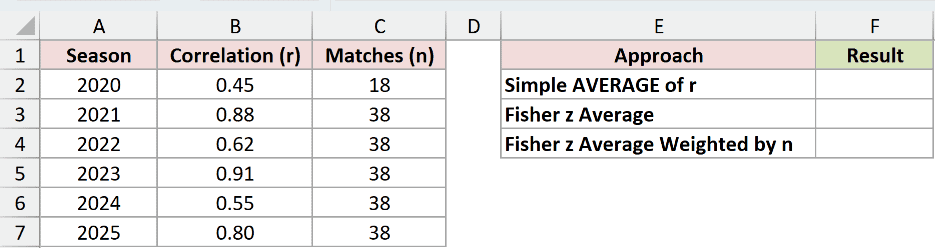
We want to combine the correlations between possession percentage and goal difference across the club’s seasons.
Start with the Fisher-scale average in F3:
=FISHERINV(AVERAGE(FISHER(B2:B7)))
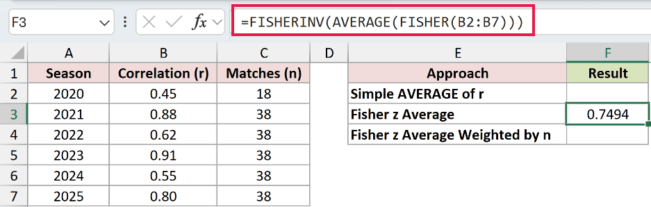
FISHER transforms every correlation, AVERAGE combines the transformed values, and FISHERINV converts back. The result is 0.7494, with every season given equal weight.
For comparison, F2 demonstrates the mistake of averaging the raw correlations directly:
=AVERAGE(B2:B7)
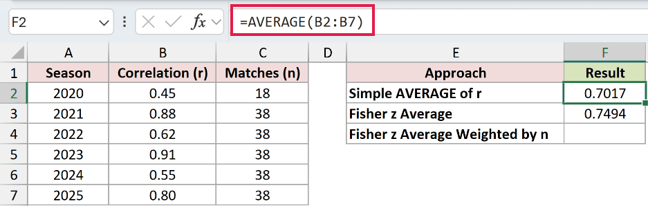
The mistaken raw average in F2 returns 0.7017. It understates the Fisher-scale average here and isn’t the method to use for this pooled estimate.
The seasons also have different sample sizes. Enter the weighted Fisher average in F4:
=FISHERINV(SUMPRODUCT(FISHER(B2:B7),C2:C7-3)/SUM(C2:C7-3))
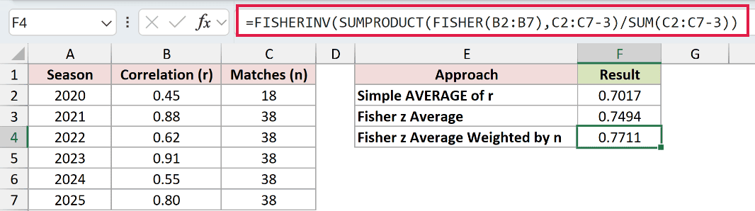
Each transformed correlation receives a weight of its match count minus 3. SUMPRODUCT adds the weighted values, and SUM provides the total weight.
The weighted result is 0.7711. The shortened 2020 season has 18 matches, while each later season has 38, so the shorter season contributes less.
Although the sheet label says “Weighted by n,” the formula uses sample size minus 3, reflecting the precision of Fisher z.
Pro Tip: In Excel 2019 and earlier, enter both F3 and F4 with Ctrl+Shift+Enter. In F3, AVERAGE receives a transformed array. In F4, SUM(C2:C7-3) needs array evaluation, although SUMPRODUCT itself does not. In current dynamic-array versions, press Enter normally.
Example 6: Plan a Correlation Study’s Sample Size
FISHER also helps estimate how much data a retail pilot needs before it starts.
Below is the dataset. Each pilot question has a target correlation, significance level, and power input. Column E will hold the required store-week count.
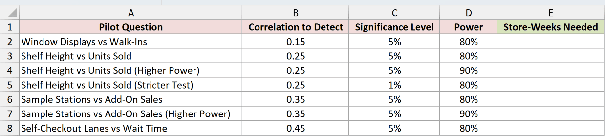
We want an approximate sample size for detecting each target correlation against zero with a two-tailed test.
Enter this formula in E2:
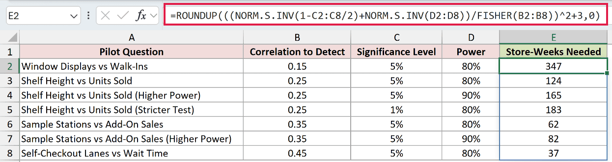
=ROUNDUP(((NORM.S.INV(1-C2:C8/2)+NORM.S.INV(D2:D8))/FISHER(B2:B8))^2+3,0)
How this formula works:
- The first NORM.S.INV uses the significance level for a two-tailed test.
- The second NORM.S.INV uses power, the chance of detecting the target relationship when it exists.
- FISHER converts the target correlation to the scale used in the sample-size approximation.
- The formula squares the ratio, adds 3, and rounds upward to a whole observation count.
Window Displays vs Walk-Ins needs 347 store-weeks to detect 0.15 at 5% significance and 80% power.
For Shelf Height vs Units Sold, detecting 0.25 needs 124 store-weeks at 80% power. Raising power to 90% increases the requirement to 165.
Keeping power at 80% but tightening significance to 1% raises that requirement to 183.
Pro Tip: Treat these as approximate counts of independent observations. Repeated weeks from the same store can be related, so a clustered or time-dependent pilot needs a design that accounts for that dependence.
Example 7: Understand FISHER Errors
The input boundaries matter most when a correlation looks perfect or arrives in the wrong format.
Below is the dataset. Column A names each scenario, column B contains the entered value, and column C is reserved for the result or deliberate error.
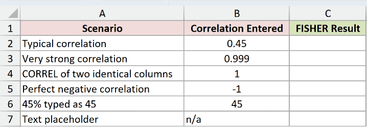
We want to see which inputs FISHER accepts and why the deliberately invalid rows fail.
Enter this formula in C2:
=FISHER(B2:B7)
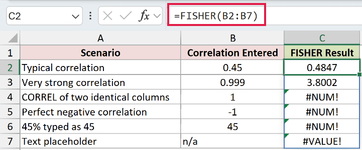
The valid input 0.45 returns 0.4847. The near-perfect input 0.999 returns 3.8002, showing how sharply FISHER stretches correlations near the boundary.
The remaining cells show errors on purpose:
- C4 returns
#NUM!: B4 contains 1, representing a perfect correlation such as CORREL would return for identical, nonconstant columns. The upper endpoint is excluded. - C5 returns
#NUM!: B5 contains -1, a perfect negative correlation. The lower endpoint is excluded too. - C6 returns
#NUM!: B6 contains 45, the mistake of typing a percentage as a whole number. Enter the intended correlation as 45% or 0.45. - C7 returns
#VALUE!: B7 contains the text placeholdern/a. Replace it with a valid correlation before calculating.
Excel evaluates each row separately, returning transformed values for valid inputs and errors for invalid inputs.
Tips & Common Mistakes
- Check blanks before transforming. In testing, a truly blank referenced cell silently returned 0. A missing correlation can therefore look like no relationship.
- Numeric text behaves differently from other text. FISHER converts a number stored as text, but a nonnumeric placeholder returns
#VALUE!. - Use FISHERINV to return to correlations. Report confidence limits and combined estimates on the correlation scale after completing the calculations on the z scale.
- ATANH is mathematically equivalent.
- Keep the spill area clear. Occupied output cells can cause
#SPILL!. Adding@forces implicit intersection instead of returning the full array. - FISHER itself works in every Excel version. The compatibility distinction is how ranges and array calculations are handled, as shown beside the examples.
I covered how FISHER transforms correlations for statistical tests, confidence intervals, and pooled estimates. I hope you found this article helpful.
Related Excel Functions / Articles:
