
Excel’s NORM.S.INV function returns the z-score whose area to the left under the standard normal curve equals a given probability.
That makes it useful when a percentile, confidence level, or upper-tail share must become a standard normal cutoff.
In this article, I’ll show you how to find critical values, set score cutoffs, calculate margins of error, and plan sample sizes.
NORM.S.INV Function Syntax in Excel
The NORM.S.INV function uses one required argument.
=NORM.S.INV(probability)
- probability (required) is the cumulative area to the left of the z-score you want. It must be greater than 0 and less than 1.
When to Use NORM.S.INV Function
- Convert percentile ranks into standard z-scores.
- Find one-tailed or two-tailed critical z values.
- Set upper-tail cutoffs for scores or performance measures.
- Calculate a normal margin of error for a proportion.
- Estimate the sample size needed for a target margin.
Example 1: Convert Percentile Ranks to z-Scores
Let’s begin by converting several student percentile ranks.
Below is the dataset. Column A lists students, column B holds percentile ranks, and the green header with empty cells in column C reserves the z-scores.
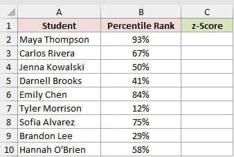
We want one z-score for each percentile rank.
Here is the spilling formula entered in C2:
=NORM.S.INV(B2:B10)
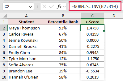
The 93% percentile rank returns 1.4758. The 41% rank returns -0.2275, while 50% returns exactly 0.
Values below 50% produce negative z-scores because they sit left of the standard normal curve’s center.
This range formula spills in Excel 2021, Excel 2024, and Microsoft 365.
In Excel 2019 and earlier, enter =NORM.S.INV(B2) in one cell and fill the formula down.
Example 2: Find One-Tailed and Two-Tailed Critical Values
Here’s a quick table for comparing the two common critical-value setups.
Below is the dataset. Column A lists confidence levels, while the green headers and empty cells in columns B and C reserve the one-tailed and two-tailed results.
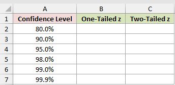
We want both critical z values for every confidence level.
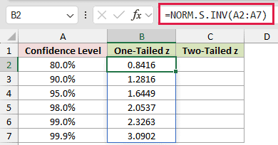
Here is the one-tailed formula entered in B2:
=NORM.S.INV(A2:A7)
Now calculate the two-tailed values in column C:
=NORM.S.INV(1-(1-A2:A7)/2)
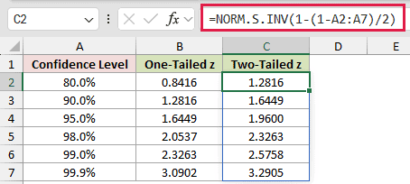
At 95% confidence, the one-tailed result is 1.6449 and the two-tailed result is 1.9600.
Two-tailed confidence splits the remaining 5% between both tails, so the cumulative probability passed to NORM.S.INV is 97.5%.
For a left-tailed cutoff, use =NORM.S.INV(1-A2:A7). The corresponding z values are negative.
Example 3: Set Top-Percent Award Cutoffs
Let’s use right-tail shares to set several exam award thresholds.
Below is the dataset. It lists award tiers and top shares.
The empty bordered cells under the green headers “z Cutoff” and “Minimum Score” are for the z cutoff and minimum score.
The table in F:G holds an exam mean of 72 and standard deviation of 9.
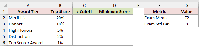
We want the z cutoff and minimum score for each award tier.
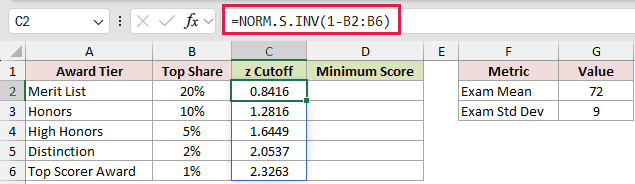
First, calculate the z cutoffs in column C:
=NORM.S.INV(1-B2:B6)
Then convert each z cutoff into an exam score:
=$G$2+C2:C6*$G$3
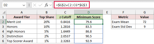
Top 5% means 95% lies to the left of the cutoff. High Honors therefore returns a z cutoff of 1.6449 and a minimum score of 86.8.
Without 1-B2:B6, passing the top share directly returns a negative cutoff for these upper-tail awards.
If you only need the raw cutoff, =NORM.INV(1-B2:B6,$G$2,$G$3) returns it in one step. The two-step version keeps the z-score visible.
Example 4: Calculate Conversion Rate Margin of Error
Here’s a practical way to use the critical z value inside a larger calculation.
Below is the dataset. Columns A to C show each landing page, visitor count, and conversion rate.
Column D holds the green Margin of Error header with empty cells below it. The 95% Confidence Level setting is in G2.
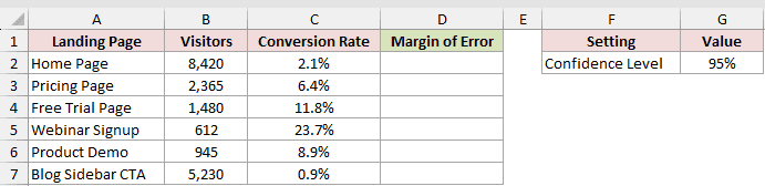
We want the normal margin of error for each conversion rate.
Here is the formula entered in D2:
=NORM.S.INV(1-(1-$G$2)/2)*SQRT(C2:C7*(1-C2:C7)/B2:B7)
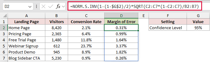
NORM.S.INV returns the two-tailed z multiplier. The SQRT portion calculates the standard error from each conversion rate and visitor count.
The Home Page’s 2.1% rate gets a 0.31% margin, producing an approximate interval from 1.79% to 2.41%.
Webinar Signup has the widest margin at 3.37% because it has the smallest visitor count and the highest conversion rate, which is closest to 50%.
Example 5: Calculate Required Sample Size
Now let’s work backward from a target margin of error.
Below is the dataset. It pairs confidence levels, target margins, and expected rates. The green header and empty cells in column D reserve the required sample sizes.
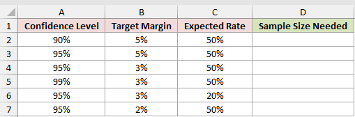
We want the minimum whole-number sample size for each planning scenario.
Here is the formula entered in D2:
=ROUNDUP((NORM.S.INV(1-(1-A2:A7)/2)/B2:B7)^2*C2:C7*(1-C2:C7),0)
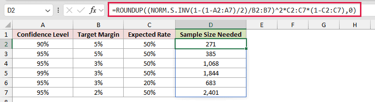
At 95% confidence, a 5% target margin and 50% expected rate require 385 observations.
Reducing the target margin to 3% raises the requirement to 1,068. With a 20% expected rate, the same settings require 683.
ROUNDUP prevents a fractional requirement from being rounded down. Use a 50% expected rate when you need the largest result for a given confidence and margin.
Example 6: Catch Probability Input Mistakes
The last example shows which probability entries work and which ones fail.
Below is the dataset. Column B mixes decimals, a percentage, alpha, a whole number, zero, and one. The result column contains empty bordered cells beneath a green header and will display z-scores or errors.
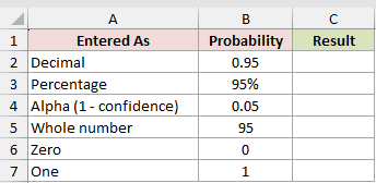
We want to see how NORM.S.INV handles each entry.
Here is the formula entered in C2:
=NORM.S.INV(B2:B7)
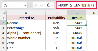
Excel stores 95% as 0.95, so the decimal and percentage rows both return 1.6449.
The alpha row contains 0.05 and returns -1.6449. The formula works correctly, but 0.05 isn’t the right input if you meant 95% confidence.
The whole number 95, zero, and one all return #NUM! because NORM.S.INV requires a probability strictly between 0 and 1.
Tips & Common Mistakes
- NORM.S.INV has been available since Excel 2010. NORMSINV is the older compatibility name.
- Remember that the probability is the cumulative area to the left. For a top share, subtract that share from 1 before using the function.
=NORM.S.DIST(NORM.S.INV(0.95),TRUE)returns 0.95, which is a handy way to check the inverse calculation.=NORM.INV(0.95,0,1)and=NORMSINV(0.95)both return the same 1.644854 result as NORM.S.INV.- A numeric text literal such as
"0.9"is converted and returns 1.2816. Ordinary nonnumeric text returns #VALUE!. - Use
=IF(OR(B2<=0,B2>=1),"Check input",NORM.S.INV(B2))when worksheet users might enter zero, one, or a whole-number percentage. =NORM.S.INV(RAND())generates a simulated standard normal value, but RAND is volatile and changes whenever Excel recalculates.- CONFIDENCE.NORM is more direct for a mean margin. With a known standard deviation, the corresponding sample-size pattern is
(z*sigma/E)^2. - Keep the spill range clear to avoid #SPILL!. Adding
@before NORM.S.INV collapses a range calculation to one result. - In Excel 2019 and earlier, use one formula per row or a legacy array formula instead of relying on a spill.
NORM.S.INV turns a left-tail probability into the standard normal cutoff that matches it.
Once the probability direction is correct, that cutoff can drive percentile conversions, confidence calculations, score thresholds, and sample-size planning.
Related Excel Functions / Articles:
