
The ISREF function in Excel checks whether an argument is a reference and returns TRUE or FALSE.
ISREF recognizes cell references, but not addresses written as text. It helps you check whether a formula produces a valid reference.
In monthly reports, you can use ISREF to check whether a worksheet exists before reading its data and show a clear message for missing tabs.
I’ll show you how to test references, check a list of sheet names, and build a revenue summary that handles missing month tabs.
ISREF Function Syntax in Excel
The ISREF function takes the argument you want to test:
=ISREF(value)
- value (required): The argument to check. It can be a cell reference, range, defined name, literal value, or expression.
ISREF tests whether the argument is a reference. It doesn’t inspect the referenced cell’s contents or convert quoted address text into a reference.
When to Use ISREF Function
- Check whether converting address text produces a valid reference.
- Check whether the worksheets listed in a report exist without using macros.
- Read data from available month tabs while labeling missing tabs.
- Check whether a lookup or another formula returns a reference.
Example 1: Test References and Address Text
Let’s start with the difference between a reference and its address written as text.
Below is the dataset. Columns D and E contain rooms and square footage. Column A labels each test, and column B will hold the ISREF results.
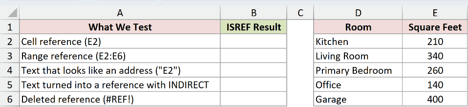
We want to see which arguments Excel recognizes as references, including the deliberate FALSE cases for address text and a deleted reference.
In B2, test the Kitchen’s square-footage cell:
=ISREF(E2)
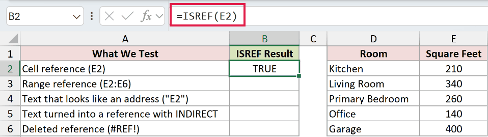
The result is TRUE. E2 contains 210, but ISREF is checking the reference to E2, not whether its contents are a number.
In B3, test the full square-footage range:
=ISREF(E2:E6)
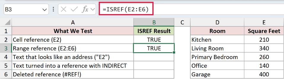
This also returns TRUE. A range is a single reference, so ISREF returns a single result. It doesn’t spill separate results for the cells inside it.
B4 is the deliberate FALSE case that passes the address as quoted text:
=ISREF("E2")
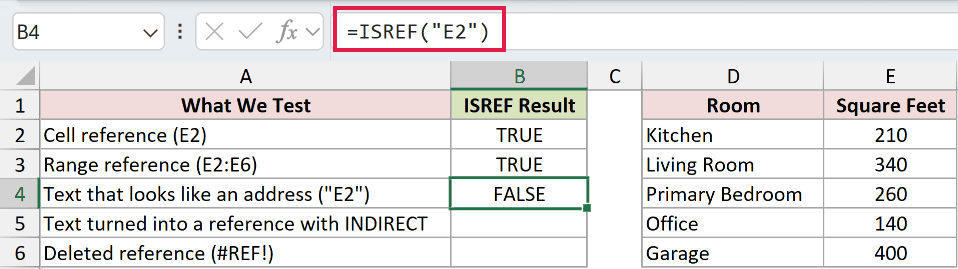
The result is FALSE because the quotation marks make “E2” text.
The INDIRECT function turns address text into a reference. In B5, use it to convert “E2” into a reference for ISREF to test:
=ISREF(INDIRECT("E2"))
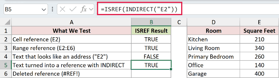
The result is TRUE. INDIRECT resolves the text to E2, so ISREF receives a reference this time.
B6 is the other deliberate FALSE case, representing a deleted reference:
=ISREF(#REF!)
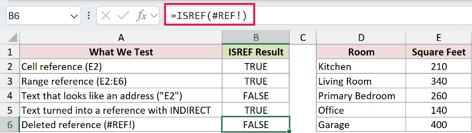
This returns FALSE. The #REF! argument is an error, so it no longer represents a valid reference.
Example 2: Check Whether Monthly Sheets Exist
Now let’s use that text-to-reference step to check worksheet names.
Below is the dataset. Column A lists month tab names from Jan through Jun, and column B is reserved for each tab’s status.
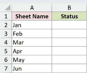
We want to check each listed tab without opening it or using a macro.
Enter this formula in B2 and copy it down through B7:
=IF(ISREF(INDIRECT("'"&A2&"'!A1")),"Sheet exists","Missing")
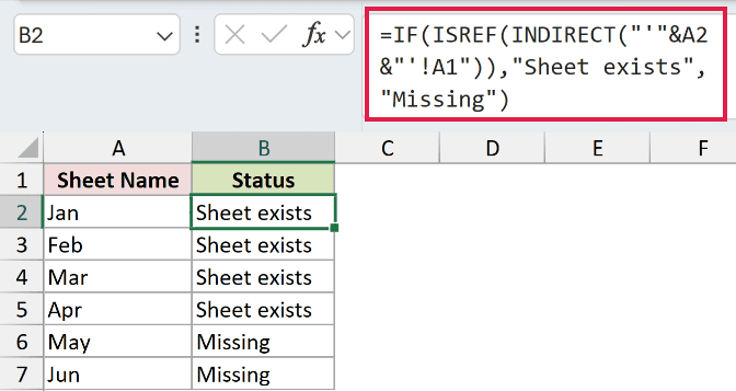
Jan, Feb, Mar, and Apr return “Sheet exists”. May and Jun return “Missing” because those tabs aren’t in the workbook.
How this formula works:
- The ampersands join the sheet name in A2 with quotation marks around the tab name and the cell address. For Jan, the resulting address text is
'Jan'!A1. - INDIRECT tries to turn that text into a reference.
- ISREF tests whether the result is a reference. IF chooses between two results based on TRUE or FALSE, so it displays “Sheet exists” or “Missing” here.
The formula is copied down, not spilled. Each row builds its own address from the adjacent sheet name.
Pro Tip: Keep the single quotes around the sheet name in the address text. That quoted form also handles tab names containing spaces.
Example 3: Summarize Revenue From Available Tabs
Let’s turn the sheet check into a working monthly summary.
Below is the dataset. Column A lists months and a year-to-date label; column B will hold revenue. The Jan through Apr tabs contain Branch and Revenue tables.
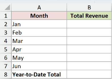
We want to total each available month’s revenue and show a message when its sheet hasn’t been added.
Enter this formula in B2 and copy it down through B7:
=IF(ISREF(INDIRECT("'"&A2&"'!A1")),SUM(INDIRECT("'"&A2&"'!B2:B6")),"No sheet yet")
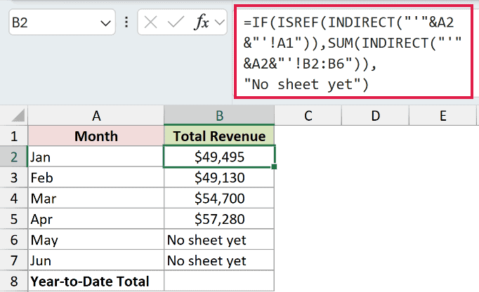
Jan returns $49,495, Feb returns $49,130, Mar returns $54,700, and Apr returns $57,280. May and Jun display “No sheet yet”.
How this formula works:
- The ISREF check tests whether A1 on the named month tab is a valid reference.
- If it is, the second INDIRECT points to B2:B6 on that tab. SUM adds numbers, so it totals the branch revenues in that range.
- If the tab is missing, IF returns the message instead of attempting that sum.
The reference to A1 checks the tab’s existence. The revenue itself comes from B2:B6, so the source tabs need the same layout.
To calculate the year-to-date total, enter this formula in B8:
=SUM(B2:B7)
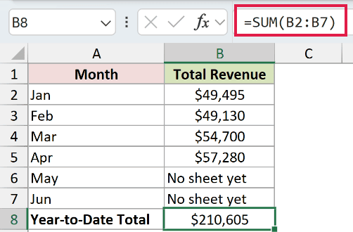
The result is $210,605. SUM adds the monthly amounts and ignores the “No sheet yet” text in the missing-month rows.
Pro Tip: IFERROR can also replace errors with a message, but it would hide errors in the revenue data too. This ISREF check only establishes whether the month tab is available.
Example 4: Check Lookup and OFFSET References
Finally, let’s check what other functions return.
Below is the dataset. Columns A and B list shipping options and costs. Column D labels the tests, and column E will hold their ISREF results.
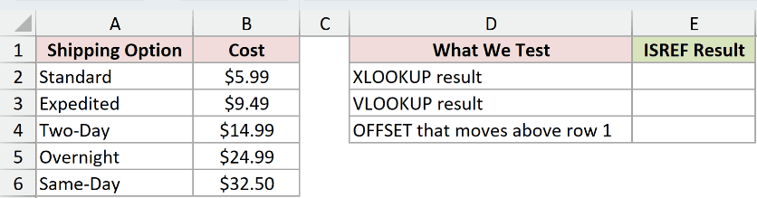
We want to compare a lookup that returns a reference with one that returns a value, then test a reference outside the worksheet.
XLOOKUP finds a match in one range and returns the corresponding item from another. In E2, use ISREF to check whether that result is a reference:
=ISREF(XLOOKUP("Two-Day",A2:A6,B2:B6))
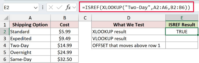
This returns TRUE. XLOOKUP returns a reference to the matching cost cell in B4. This example requires Excel 2021 or later because it uses XLOOKUP.
VLOOKUP searches the first column of a table and returns a value from another column in the matching row. In E3, compare its result using ISREF:
=ISREF(VLOOKUP("Two-Day",A2:B6,2,FALSE))
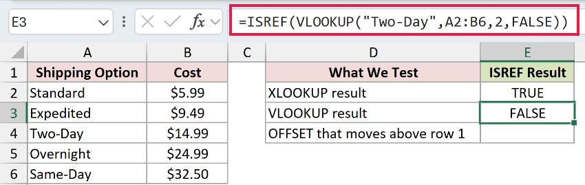
The comparison returns FALSE. VLOOKUP finds the matching shipping cost, but returns its value rather than a reference. FALSE here doesn’t mean the lookup failed.
OFFSET returns a reference a specified number of rows and columns from a starting cell. ISREF can test whether that destination is valid.
In E4, deliberately request a destination above the worksheet’s first row:
=ISREF(OFFSET(B2,-2,0))
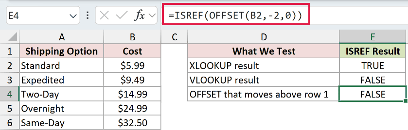
This returns FALSE because the requested position falls outside the worksheet. OFFSET can return a reference, but the destination must be valid.
Tips & Common Mistakes
- Don’t use ISREF to validate cell contents. A valid reference says nothing about whether the referenced data is complete or suitable for your calculation.
- Quoted addresses need conversion. ISREF doesn’t turn address text into a reference. INDIRECT handles that step in the examples above.
- A range isn’t a list of separate tests. ISREF checks the range as a single reference. Copy the monthly formulas down to check each sheet name separately.
- Defined names must refer to references. A name pointing to a worksheet range can be tested with ISREF. Don’t assume every defined name represents a range.
- Check the source layout as well as the tab name. The revenue summary assumes each available sheet stores branch revenue in B2:B6. A sheet-existence check can’t confirm that layout.
- ISREF works in every version of Excel. Companion functions may have their own version requirements, as XLOOKUP does in the final example.
These examples covered reference tests, sheet-existence checks, and a revenue summary that labels missing tabs.
The lookup and OFFSET tests showed how ISREF handles returned values, valid references, and invalid destinations.
Related Excel Functions / Articles:
