
The NEGBINOM.DIST function in Excel returns the probability of a given number of failures before you reach a target number of successes.
For example, you might keep submitting grant applications until you receive enough awards. The function measures how many rejections you could encounter along the way.
You supply the number of unsuccessful attempts, not the total attempts. The success target goes in a separate argument.
I’ll compare the chance of a sale on a particular test drive with the chance of selling by then, and check whether an interview budget covers a hiring target.
NEGBINOM.DIST Function Syntax in Excel
The function takes four required arguments:
=NEGBINOM.DIST(number_f, number_s, probability_s, cumulative)
- number_f is the number of failures before the target success. Use a nonnegative whole number.
- number_s is the target number of successes. Use a positive whole number.
- probability_s is the success probability for each attempt. Use a value strictly between 0 and 1.
- cumulative controls the question:
FALSEreturns the probability of exactly that many failures;TRUEreturns the probability of at most that many failures.
The model assumes independent attempts with the same success probability each time. A success means the outcome you’re counting, such as an award, purchase, or sign-up.
When to Use NEGBINOM.DIST Function
- Build a probability table showing unsuccessful contacts before a sign-up target.
- Estimate the chance of exceeding a rejection limit before receiving enough awards.
- Calculate the chance that a first purchase happens on, or by, a particular attempt.
- Check whether an interview or visitor budget is likely to cover a target.
Example 1: Build a Failure Probability Table
Let’s start with a charity canvasser working toward a sign-up target.
Below is the dataset. Column A lists doors without a sign-up, E2 and F2 hold the target and rate, and columns B and C will show probabilities.
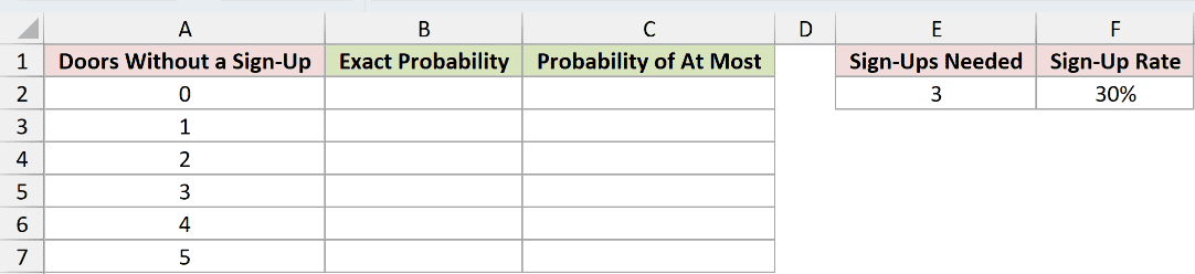
We want the probability of each failure count before the third sign-up, assuming a 30% sign-up rate at every door.
Enter this formula in B2:
=NEGBINOM.DIST(A2:A7,E2,F2,FALSE)
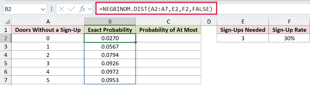
The formula spills into B2:B7. Each result measures exactly the failure count beside it, with the third sign-up completing the sequence.
For 0 failures, B2 returns 0.0270. For 5 failures, B7 returns 0.0953.
Range formulas spill in Excel 2021, Excel 2024 and Microsoft 365. In Excel 2019 and earlier, use a single-row reference and copy the formula down.
Now enter the cumulative version in C2:
=NEGBINOM.DIST(A2:A7,E2,F2,TRUE)
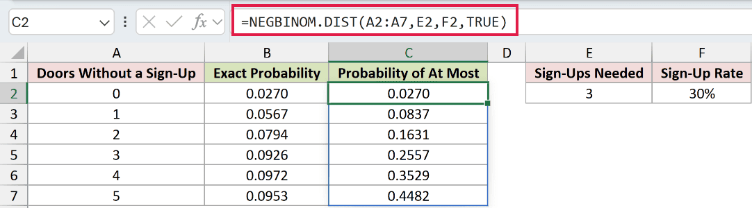
This formula spills into C2:C7. TRUE adds the probabilities from zero failures through the count in each row.
For 5 failures, C7 returns 0.4482. That’s the probability of reaching the third sign-up with at most 5 unsuccessful doors along the way.
The exact and cumulative results both start at 0.0270 because there are no failure counts below zero to include.
Pro Tip: Keep the output cells below each formula empty. An occupied cell can cause #SPILL!, a spill error, because Excel needs room for the whole probability column.
Example 2: Compare Exactly, At Most, and More
A grant application plan needs different answers depending on how you phrase the rejection limit.
Below is the dataset. B1:B3 contain the award target, approval rate, and rejection count. The labeled answer cells B4:B6 are empty for now.
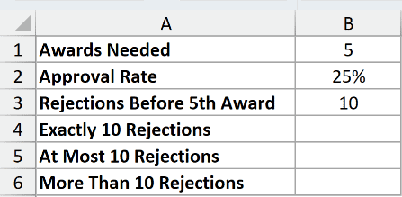
We want to compare exactly, at most, and more than 10 rejections before the fifth award, using a 25% approval rate.
For exactly that rejection count, enter this in B4:
=NEGBINOM.DIST(B3,B1,B2,FALSE)
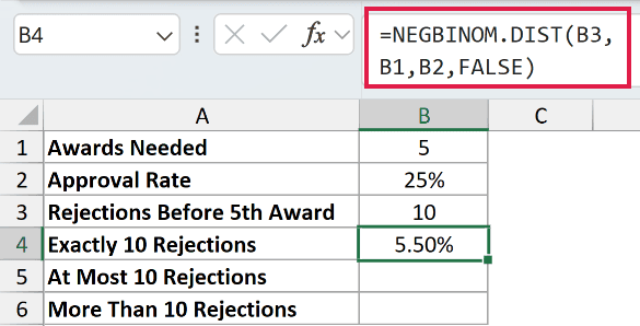
B4 returns 5.50%. This covers sequences ending at the fifth award with exactly 10 rejections before it.
For at most that many rejections, enter this in B5:
=NEGBINOM.DIST(B3,B1,B2,TRUE)
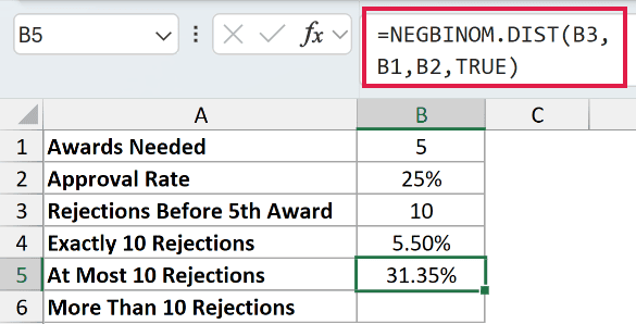
B5 returns 31.35%. This includes every qualifying sequence with fewer rejections as well as those with exactly 10.
For the chance of exceeding the limit, enter this in B6:
=1-B5
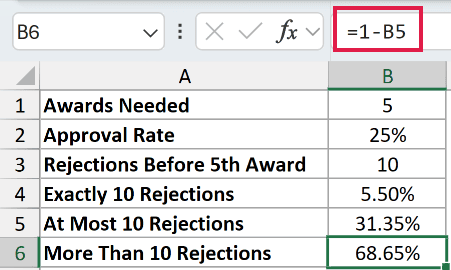
B6 returns 68.65%. Subtracting the cumulative probability from 1 leaves the chance of more than 10 rejections before the target award.
Subtracting the exact probability gives the chance of any failure count except the specified count. Use the cumulative result for this upper-tail calculation.
Example 3: Find the First-Sale Probability
For a first sale, the success target is one. This is called the geometric case of the negative binomial distribution.
Below is the dataset. B1 contains the purchase rate and B2 the test-drive number. B3:B6 are ready for the calculations below.
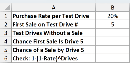
We want the chance of a first sale on test drive 5, then the chance of making a sale by that drive.
First, convert the drive number to failures in B3:
=B2-1
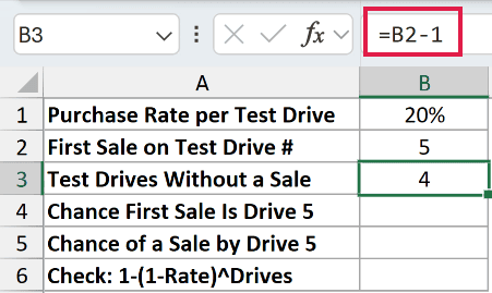
B3 returns 4. A first sale on drive 5 requires 4 unsuccessful drives before it, so entering the drive number directly as failures would be a mistake.
For the first sale on that drive, enter this in B4:
=NEGBINOM.DIST(B3,1,B1,FALSE)
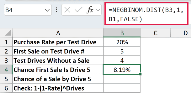
At the 20% purchase rate in B1, B4 returns 8.19%. The final argument restricts the result to exactly the failure count in B3.
For a sale by that drive, enter this in B5:
=NEGBINOM.DIST(B3,1,B1,TRUE)
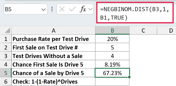
B5 returns 67.23%. This includes a first sale on any drive up to and including drive 5.
The formula in B6 is a cross-check of that cumulative answer:
=1-(1-B1)^B2
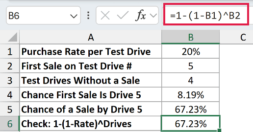
The cross-check also returns 67.23%. Start with 1 and subtract the chance of no purchase throughout the drives to get the chance of at least one sale.
This shortcut works here because we’re waiting for the first success. For a larger success target, use the full distribution calculation.
Example 4: Check an Interview Budget
Now let’s apply the attempt-limit calculation to several hiring plans at once.
Below is the dataset. Columns A:D contain roles, hires needed, pass rates, and interview budgets. Column E will show the chance of filling each role within budget.

We want the probability of reaching each hiring target before its interview allowance runs out.
Enter this formula in E2:
=NEGBINOM.DIST(D2:D6-B2:B6,B2:B6,C2:C6,TRUE)
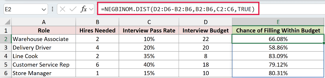
The formula spills into E2:E6, using each role’s own inputs.
How this formula works:
D2:D6-B2:B6subtracts the required hires from the interview budget, leaving the allowed failures.B2:B6supplies each success target, whileC2:C6supplies its pass rate.TRUEincludes every failure count up to the allowance, so finishing early also counts.
The Warehouse Associate plan needs 2 hires within 22 interviews at a 10% pass rate. Its probability is 66.08%.
Delivery Driver returns 58.86%, Line Cook returns 83.09%, Customer Service Rep returns 79.12%, and Store Manager returns 80.31%.
Here, a successful interview is assumed to produce a hire. If passing and accepting an offer are separate hurdles, the input rate must reflect the outcome you’re counting.
Example 5: Cross-Check With BINOM.DIST
You can describe the same visitor budget by counting failures before the target or purchases within a fixed number of visits.
Below is the dataset. B1:B3 hold purchases needed, purchase rate, and visitor budget. B4:B7 are empty spaces for the probability checks and averages.
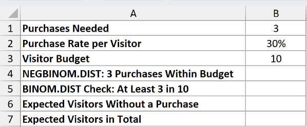
We want the chance of reaching 3 purchases within 10 visitors at a 30% purchase rate, then the average visitors needed to reach that target.
Enter the NEGBINOM.DIST formula in B4:
=NEGBINOM.DIST(B3-B1,B1,B2,TRUE)
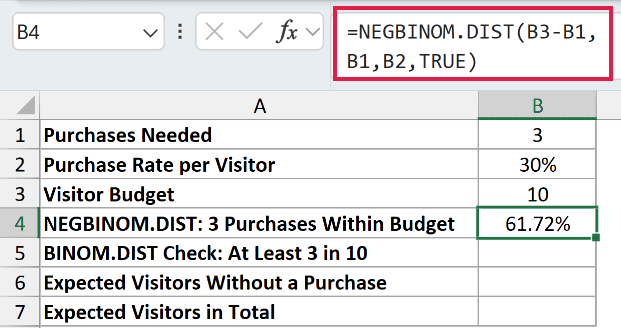
B4 returns 61.72%. Subtracting the purchase target from the visitor budget converts total attempts to the failure allowance.
For the matching BINOM.DIST cross-check, enter this in B5:
=1-BINOM.DIST(B1-1,B3,B2,TRUE)
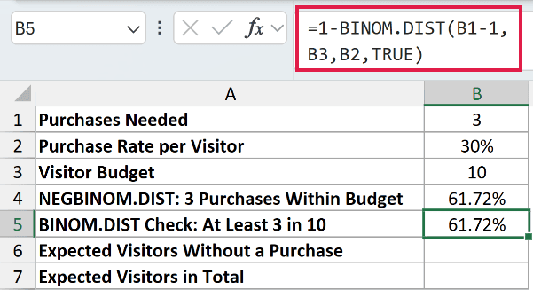
The cross-check returns the same 61.72%. BINOM.DIST calculates the chance of falling short of the purchase target within the fixed visitor budget; subtraction leaves meeting or exceeding it.
Next, calculate the expected visitors without a purchase in B6:
=B1*(1-B2)/B2
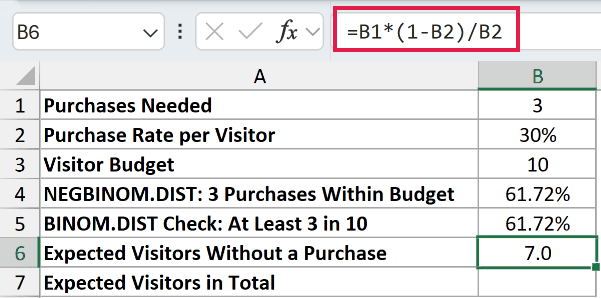
B6 returns 7.0. This is the average number of unsuccessful visits before reaching the purchase target across repeated runs of the model.
For the expected total visitors, enter this in B7:
=B1/B2
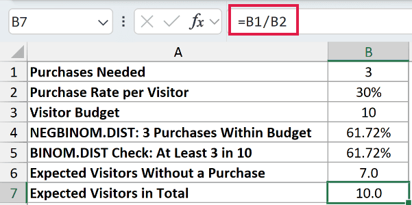
B7 returns 10.0. This expected total includes the visitors who purchase as well as those who don’t.
An average of 10.0 visitors doesn’t guarantee completion within that budget. The probability of doing so remains 61.72%, as B4 and its cross-check show.
Tips & Common Mistakes
- Count failures separately from attempts. Subtract the success target from a total-attempt allowance before passing it as
number_f. - Keep all four arguments. Omitting
cumulativeis rejected at formula entry. ChooseFALSEfor exactly orTRUEfor at most. - Check the argument limits. In testing, a negative failure count, a success target of 0, or a success probability of 0 or 1 returned
#NUM!. - Use whole-number counts. Excel truncates decimal failure and success counts. In testing, 10.9 failures and 5.9 successes were treated as 10 and 5.
- Choose a rate that fits the model. These probabilities assume independent attempts and an unchanged success rate.
- Match the function to the count. POISSON.DIST models event counts over a fixed interval, such as arrivals during a shift. NEGBINOM.DIST counts failures while waiting for a success target.
- An inverse binomial question uses a fixed trial count. BINOM.INV finds the smallest success count whose cumulative probability reaches a chosen threshold. It doesn’t find the attempts needed for your target.
- The older function name still works. NEGBINOM.DIST is available in Excel 2010 and later. The older NEGBINOMDIST remains for compatibility and calculates exact probabilities only.
Related Excel Functions / Articles:
