
The TBILLPRICE function in Excel returns a Treasury bill’s price per $100 of face value from its settlement date, maturity date, and discount rate.
Face value is the amount repaid at maturity. The returned price tells you how much you pay for that amount, so larger purchases need a separate scaling step.
The discount rate measures the discount against face value. It isn’t the same as the return measured against your purchase cost.
I’ll show you how to price different bill terms, calculate purchase costs, and catch rate-entry mistakes that Excel accepts without an error.
TBILLPRICE Function Syntax in Excel
TBILLPRICE requires each of these arguments:
=TBILLPRICE(settlement, maturity, discount)
- settlement (required): The date you settle the purchase of the Treasury bill.
- maturity (required): The date the bill pays its face value. It must follow settlement and be no more than one calendar year later.
- discount (required): The annual discount rate, entered as a percentage or its decimal equivalent. It must be greater than zero.
TBILLPRICE uses the actual days between the dates and a 360-day year. There is no basis argument to change that convention.
When to Use TBILLPRICE Function
- Convert a quoted discount rate into a price per $100 of face value.
- Compare bill terms while keeping the settlement date and discount rate fixed.
- Calculate purchase costs for different face amounts.
- See how changing discount rates affect the price of the same bill.
Example 1: Price a 13-Week Treasury Bill
Let’s start with a bill’s dates and its quoted discount rate.
Below is the dataset with settlement, maturity, and discount-rate inputs in B1:B3. The labelled result cell B4 will hold the price per $100 face value.
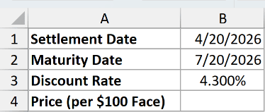
We want the price of the bill settling on 4/20/2026 and maturing on 7/20/2026 at a 4.300% discount rate.
Enter this formula in B4:
=TBILLPRICE(B1,B2,B3)
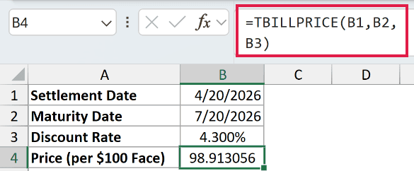
The result is 98.913056 per $100 of face value. It is a price, so don’t format the result as a percentage.
The dates are 91 days apart. TBILLPRICE applies the annual discount rate to that fraction of its 360-day year, then subtracts the discount from face value.
For a larger purchase, you still start with this per-$100 quote. Example 3 converts it into the actual purchase cost.
Example 2: Compare Prices Across Bill Terms
Now let’s keep the rate fixed and change how long the money stays invested.
Below is the dataset with bill terms in A:B, maturity and price columns in C:D, and settlement and discount-rate inputs in G2:G3.

We want to calculate each maturity date, then price every bill using the same settlement date and discount rate.
First, enter the maturity-date formula in C2 and copy it down through C5:
=$G$2+B2*7
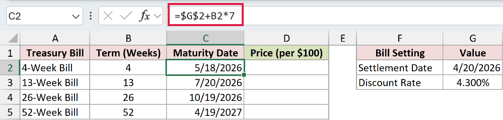
The multiplication converts weeks to days, which Excel adds to settlement. The dollar signs keep G2 fixed as the term reference changes down the column.
The maturity dates are 5/18/2026, 7/20/2026, 10/19/2026, and 4/19/2027.
Next, enter this formula in D2 and copy it down through D5:
=TBILLPRICE($G$2,C2,$G$3)
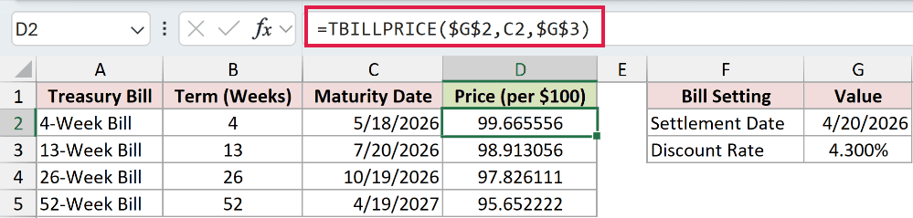
Each row uses its own maturity date from column C, while the settlement date and 4.300% discount rate stay fixed.
The prices per $100 are:
- 4-week bill: 99.665556.
- 13-week bill: 98.913056.
- 26-week bill: 97.826111.
- 52-week bill: 95.652222.
At the same discount rate, a longer term produces a larger discount and a lower purchase price.
These are copied-down formulas. Passing a bare range to TBILLPRICE doesn’t calculate the whole column; Example 5 shows the array conversion needed for that.
Example 3: Calculate the Actual Purchase Cost
A per-$100 quote needs scaling when your face amount changes.
Below is the dataset with face amounts in column A, a Purchase Cost column in B, and a bill-input card in D:E with a labelled price cell.
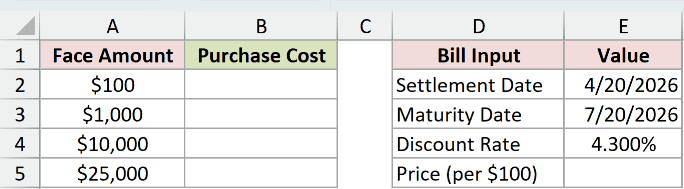
We want the cash needed to buy each face amount using the bill’s calculated price.
First, calculate the price per $100 in E5:
=TBILLPRICE(E2,E3,E4)
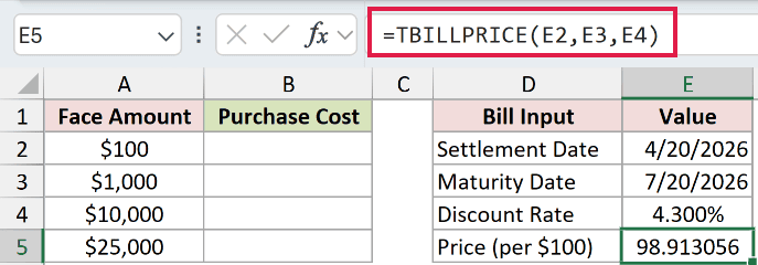
The price cell displays 98.913056. We’ll reference this cell directly when calculating each purchase cost.
Enter the following formula in B2 and copy it down through B5:
=$E$5/100*A2
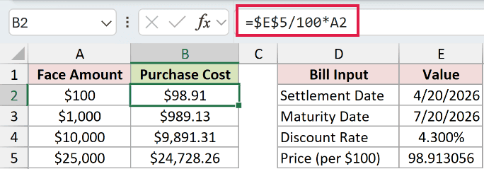
Dividing the quote by 100 converts it to a price per dollar of face value. Multiplying by column A scales it to your purchase.
The resulting costs are:
- $100 face amount: $98.91.
- $1,000 face amount: $989.13.
- $10,000 face amount: $9,891.31.
- $25,000 face amount: $24,728.26.
The face amount is what the bill repays at maturity. The Purchase Cost column shows the smaller amount paid at settlement.
Pro Tip: Reference E5 instead of typing its displayed price into the cost formula. This keeps the calculation tied to the underlying value when you change the dates or rate.
Example 4: Catch the Whole-Number Rate Mistake
A missing percent sign can produce a price that looks like a valid answer.
Below is the dataset comparing a correctly entered percentage with a deliberately wrong whole-number rate. Dates are in F2:F3, and column C holds the price calculations.

We want to see how the incorrect rate entry changes the price without triggering an Excel error.
Enter this formula in C2, then copy it to C3 for the deliberate mistake row:
=TBILLPRICE($F$2,$F$3,B2)

The correctly entered 4.25% in B2 returns 99.268056 in C2.
The incorrect rate entry of 4.25 in B3 produces 26.805556 in C3.
Excel accepts the whole number as the discount argument. It doesn’t know you meant a percentage, so the incorrect input produces no error.
Re-enter the mistaken rate with its percent sign.
Example 5: Compare Discount Rates With One Formula
You can also price several rate scenarios without copying TBILLPRICE down the column.
Below is the dataset with discount-rate scenarios in A2:A5, a price column in B, and fixed settlement and maturity dates in E2:E3.
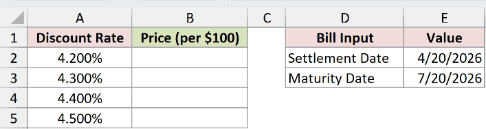
We want a separate price for each discount rate while keeping the bill’s dates unchanged.
Enter this formula in B2:
=TBILLPRICE(E2,E3,+A2:A5)
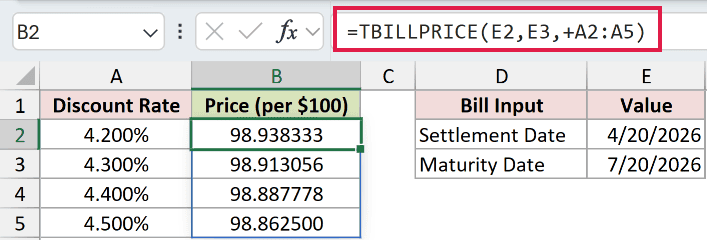
The leading + converts the rate range into a calculated numeric array that TBILLPRICE can process. The results spill automatically into B2:B5.
Passing a bare range to TBILLPRICE produces a single #VALUE! error. The plus sign is what makes this range-based calculation work.
This spilling formula works in Excel 2021, Excel 2024, and Microsoft 365. In Excel 2019 and earlier, use individual rate references and copy down, as in Example 4.
The scenario results are:
- 4.200%: 98.938333.
- 4.300%: 98.913056.
- 4.400%: 98.887778.
- 4.500%: 98.862500.
With the dates fixed, increasing the discount rate lowers the price. You can change the input rates to update the comparison.
Example 6: Check Date Limits and Input Errors
Let’s finish with valid inputs beside deliberate error cases.
Below is the dataset with case labels, settlement dates, maturity dates, and discount rates. Column E holds the price or intentional error for each case.
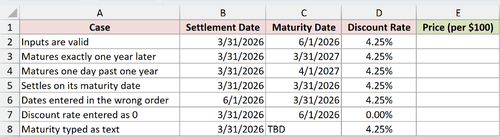
We want to check the calendar-year boundary and identify which invalid inputs TBILLPRICE rejects.
Enter this formula in E2 and copy it down through E8:
=TBILLPRICE(B2,C2,D2)
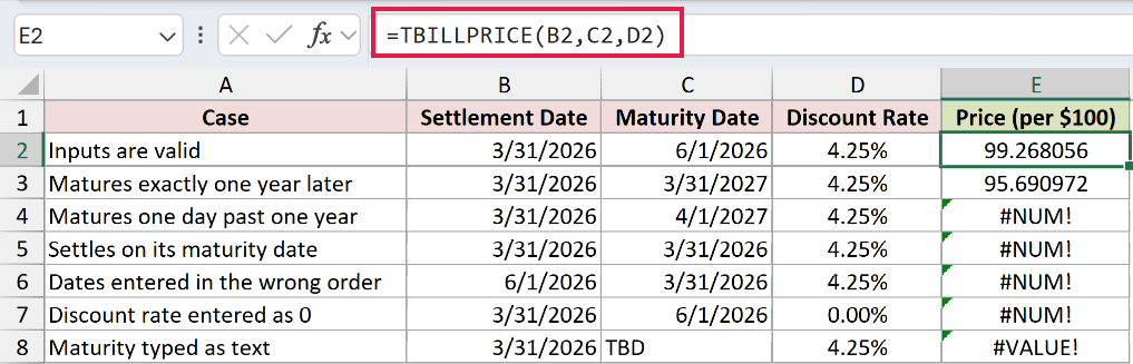
The valid starting case returns 99.268056 in E2. The bill maturing exactly one calendar year later, on 3/31/2027, returns 95.690972 in E3.
The remaining rows deliberately demonstrate rejected inputs:
E4, one day past one year:#NUM!. The maturity date of 4/1/2027 is beyond the allowed window from 3/31/2026.E5, settlement equals maturity:#NUM!. Settlement must come before maturity.E6, reversed dates:#NUM!. Correct the settlement and maturity entries so they are in chronological order.E7, zero discount:#NUM!. The rate shown as 0.00% is invalid; use a positive discount rate.E8, text maturity:#VALUE!. Replace the placeholderTBDwith the actual maturity date.
The error cells are demonstrations, even though they sit in the result column. Fix each input problem before treating that row as a usable price.
Tips & Common Mistakes
- Use settlement for this purchase. If you’re buying an existing bill, calculate from your settlement date to its maturity date.
- Keep price and face amount separate. TBILLPRICE returns a quote per $100 face value. Scale it before treating it as the cash cost of a larger purchase.
- Check the discount input. A positive number can still be the wrong rate. The whole-number mistake in Example 4 shows why an error-free formula isn’t enough.
- Use date cells. Excel can parse some text dates, but a placeholder isn’t a date. Any time portions in settlement or maturity are truncated.
- Respect the calendar-year limit. Maturity must follow settlement and fall within one calendar year. The 360-day pricing convention doesn’t change that date limit.
TBILLPRICE lets you turn a quoted discount rate into a Treasury bill price you can use in a purchase worksheet.
Revisit Example 5 when you want to compare prices across several discount-rate scenarios.
Other Excel articles you may also like:
