
Excel’s T.DIST.RT function returns the probability to the right of a t statistic on Student’s t distribution.
Use it when you’ve calculated a t statistic and want a one-tailed p-value for a claim that a mean has increased or exceeds a target.
A negative t statistic is valid, but its right-tail probability answers a different question from whether the mean has fallen.
I’ll show you how to calculate p-values from a table, build a test from raw data, and handle negative statistics without changing the claim you’re testing.
T.DIST.RT Function Syntax in Excel
T.DIST.RT takes the statistic and its degrees of freedom:
=T.DIST.RT(x,deg_freedom)
- x (required): The t statistic at which to calculate the right-tail probability. Negative values are allowed.
- deg_freedom (required): The degrees of freedom for the test. Excel truncates decimals, and values below 1 return
#NUM!.
Degrees of freedom describe how much independent information the test uses. The appropriate value depends on how you calculated the statistic.
T.DIST.RT is available in Excel 2010 and later.
When to Use T.DIST.RT Function
- Convert existing t statistics into right-tailed p-values for feature or product tests.
- Test whether a sample mean exceeds a specified target.
- Compare a right-tailed p-value with your chosen significance threshold.
- Check how the direction of a claim changes the probability you need.
Example 1: Calculate p-Values for Feature Tests
Let’s start with feature tests whose t statistics have already been calculated.
Below is the dataset. Columns A:C contain feature names, t statistics, and degrees of freedom. Column D will hold the one-tailed p-values.
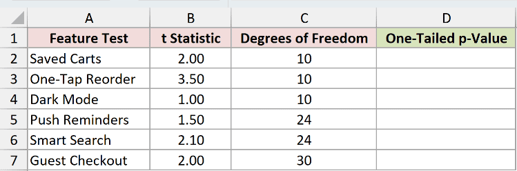
We want the right-tailed p-value for each feature’s proposed increase.
Enter this formula in D2:
=T.DIST.RT(B2:B7,C2:C7)
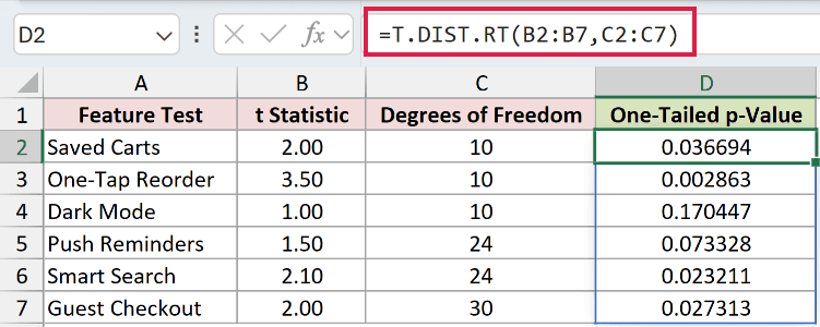
The formula pairs each statistic in B2:B7 with the degrees of freedom on the same row in C2:C7. Results spill into D2:D7.
Saved Carts returns 0.036694, while One-Tap Reorder returns 0.002863. Dark Mode returns 0.170447, so its statistic is less unusual under the no-increase assumption.
Push Reminders returns 0.073328, Smart Search returns 0.023211, and Guest Checkout returns 0.027313.
Notice that Saved Carts and Guest Checkout both have a t statistic of 2.00. Their different degrees of freedom produce different p-values.
This range formula spills in Excel 2021, Excel 2024, and Microsoft 365. In Excel 2019 and earlier, use individual row references and copy down.
Example 2: Test a Mean Against a Target
Now let’s calculate the statistic ourselves from trainee assembly counts.
Below is the dataset. Columns A:B list trainees and units assembled. The D:E card contains the target input and labelled spaces for the test calculations.
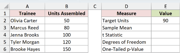
We want to test whether the mean output exceeds the target of 90 units, entered in E2.
First, use AVERAGE, which calculates the sample mean, in E3:
=AVERAGE(B2:B6)
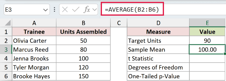
The sample mean is 100.00. Next, we need to express its distance above the target relative to the uncertainty in that mean.
STDEV.S calculates the sample standard deviation, COUNT counts numeric observations, and SQRT returns a square root. Together, they calculate the standard error used in the t statistic.
Enter the t-statistic formula in E4:
=(E3-E2)/(STDEV.S(B2:B6)/SQRT(COUNT(B2:B6)))
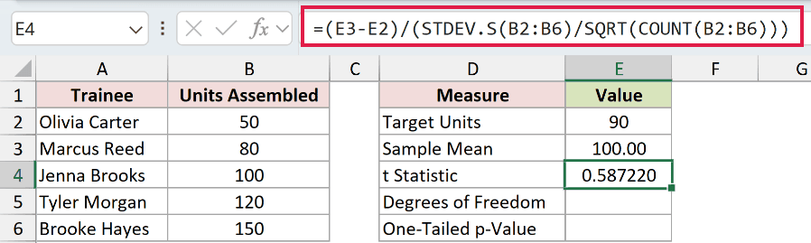
How this formula works:
- The numerator subtracts the target in E2 from the sample mean in E3.
- The denominator divides the sample standard deviation by the square root of the observation count.
- Dividing the difference by that standard error returns the t statistic, 0.587220.
For this one-sample test, degrees of freedom are the observation count minus one. Enter this in E5:
=COUNT(B2:B6)-1
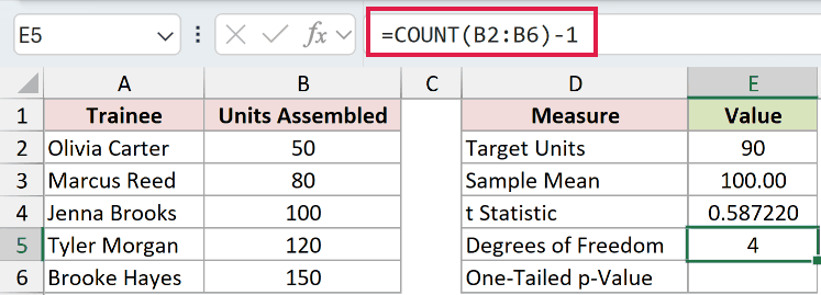
E5 returns 4. We can now use the statistic and degrees of freedom to calculate the right-tailed p-value in E6:
=T.DIST.RT(E4,E5)
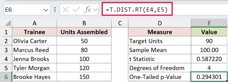
The p-value is 0.294301. Although the sample mean exceeds the target, this result doesn’t provide evidence of an increase at a significance threshold of 0.05.
Pro Tip: Reference the calculated statistic in E4 directly. Retyping the displayed value rounds the input before T.DIST.RT calculates the probability.
Example 3: Compare p-Values With a Cutoff
Let’s turn battery-trial p-values into decisions and check the matching critical t value.
Below is the dataset. Column A names the battery formulations being tested, and B holds their t statistics. Columns C:D will show results.
The F:G card holds settings and spaces for cutoff checks.

We want to test each proposed increase against alpha, the significance threshold entered in G2, using the shared degrees of freedom in G3.
Enter the p-value formula in C2:
=T.DIST.RT(B2:B4,G3)
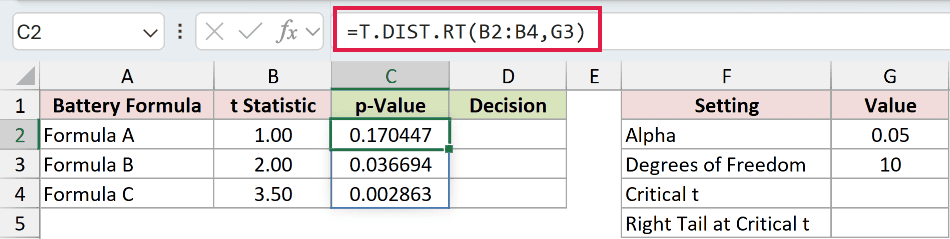
C2:C4 returns 0.170447, 0.036694, and 0.002863. The threshold in G2 is 0.05, and G3 contains 10 degrees of freedom.
IF checks a condition and returns the matching text. Here, it labels whether each T.DIST.RT result meets the rejection threshold.
Enter this formula in D2:
=IF(C2:C4<=G2,"Reject H0","Keep H0")
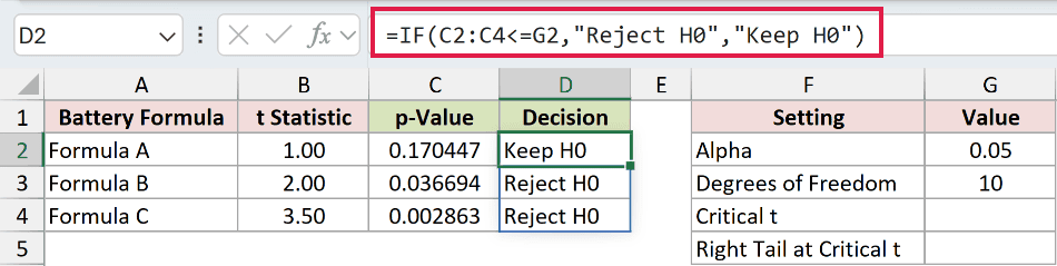
The decisions spill into D2:D4: Keep H0, Reject H0, and Reject H0.
H0 means the null hypothesis, the baseline claim of no increase. The worksheet’s “Keep H0” label means insufficient evidence to reject it, not proof that it’s true.
For a comparison using the statistic itself, T.INV returns the t value with a specified probability to its left. This lets us find the matching rejection cutoff.
Enter this comparison formula in G4:
=T.INV(1-G2,G3)
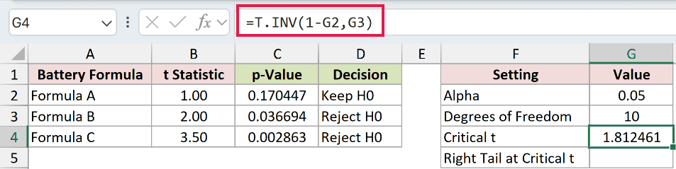
The critical t is 1.812461. Subtracting alpha from one supplies the left-tail probability, leaving alpha in the right tail.
Formula B’s statistic of 2.00 and Formula C’s 3.50 exceed that cutoff. This comparison agrees with their p-value decisions.
To check the cutoff’s right-tail probability, enter this in G5:
=T.DIST.RT(G4,G3)
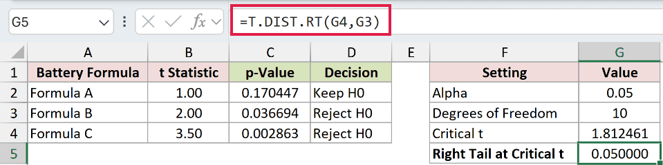
The check returns 0.050000, matching alpha. It confirms that the p-value threshold and critical t comparison describe the same right-tailed test.
Example 4: Match the Tail to the Claim
A negative statistic doesn’t cause an error, but it makes the direction of your claim especially important.
Below is the dataset. Columns A:D contain delivery checks, claims, signed statistics, and degrees of freedom. Column E will hold the probabilities for comparison.

We want to compare the evidence for delivery times above the target with the evidence for times below it.
For the slower route’s “Mean time > 30 min” claim, enter this in E2:
=T.DIST.RT(C2,D2)
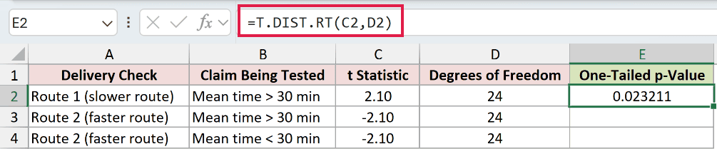
The positive statistic 2.10 returns 0.023211. This is a small right-tail probability for the claim that the mean time exceeds the target.
The next row is a direction comparison: it tests the same “greater than” claim using the faster route’s negative statistic. Enter this in E3:
=T.DIST.RT(C3,D3)
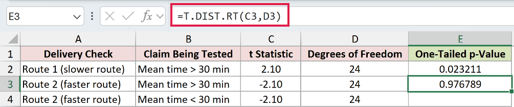
This comparison returns 0.976789 for -2.10. The large probability is correct for the displayed claim, but using it to judge faster delivery would test the wrong direction.
For the “Mean time < 30 min” claim, reverse the statistic’s sign before calculating the right tail. Enter this in E4:
=T.DIST.RT(-C4,D4)
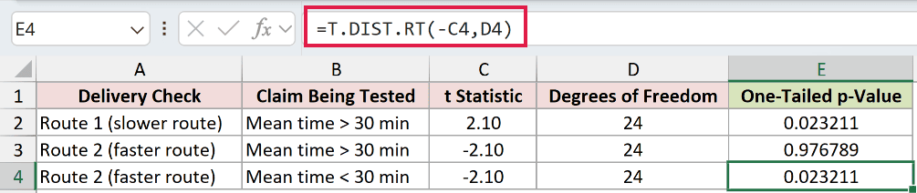
The result is 0.023211. Because the t distribution is symmetric, the right tail at the reversed statistic equals the left tail at the original statistic.
These formulas stay separate by row because the final row changes direction. Copying the first formula through every row would miss that change.
Pro Tip: Choose the claim’s direction before examining the result. Automatically making every statistic positive selects the smaller tail and can turn evidence against your claim into apparent support.
Example 5: Check Degrees of Freedom
Finally, let’s check decimal degrees of freedom and compare a large-df result with the normal distribution.
Below is the dataset. Column A contains degrees of freedom, column B will hold right-tail probabilities, and the D:E card provides a normal-distribution comparison.
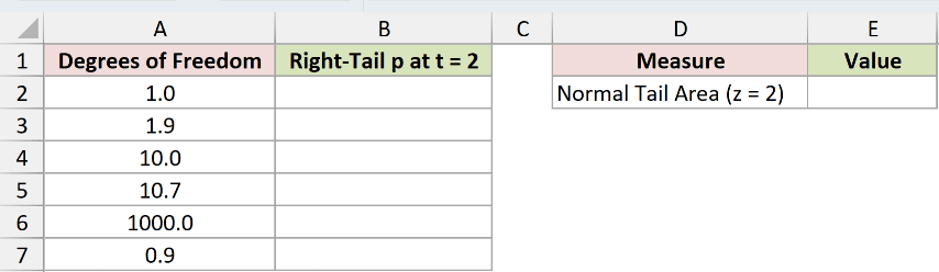
We want to hold the t statistic at 2 and see how each degrees-of-freedom input affects the result.
Enter this formula in B2:
=T.DIST.RT(2,A2:A7)
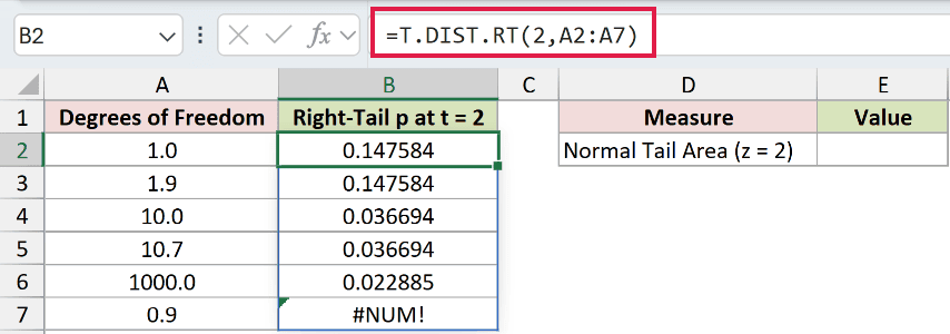
The results spill into B2:B7, including the deliberate error in the final row.
- Degrees of freedom 1.0 and 1.9 both return 0.147584. Excel truncates the decimal part.
- 10.0 and 10.7 both return 0.036694 for the same reason.
- 1000.0 returns 0.022885, closer to the normal-tail comparison.
- 0.9 deliberately returns #NUM! in B7 because degrees of freedom below 1 are invalid. Correct the input; this isn’t a probability result.
NORM.S.DIST calculates a standard normal probability. We’ll use its cumulative left tail at a negative value as the symmetric right-tail comparison for T.DIST.RT.
Enter the comparison formula in E2:
=NORM.S.DIST(-2,TRUE)
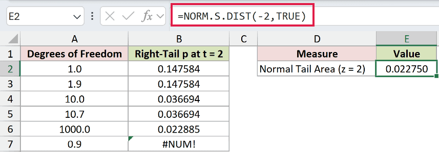
The normal comparison returns 0.022750. T.DIST.RT’s 0.022885 at the largest degrees of freedom shown is close, but the displayed results still differ.
This comparison illustrates how the t distribution approaches the normal distribution as degrees of freedom increase. Keep the degrees of freedom appropriate to your actual test.
Tips & Common Mistakes
- Keep the sign of the t statistic. A right-tail probability for a negative statistic is valid; the claim determines whether you need that tail or the opposite one.
- T.DIST.RT needs only the statistic and degrees of freedom. Don’t add a cumulative argument.
- Numeric text such as
"2"is accepted, but nonnumeric text such as"abc"returns#VALUE!. Check imported inputs before calculating. - A blank statistic is treated as zero. Make sure a missing statistic isn’t being mistaken for a completed test.
- Keep output cells empty for range formulas. A blocked spill prevents Excel from placing the results, and adding
@can reduce a range calculation to a single result. - A p-value measures how unusual the statistic is under the null hypothesis and test assumptions. It isn’t the probability that your claim is true.
The examples covered table-based p-values, a test from raw data, and cutoff comparisons.
They also showed how claim direction and degrees of freedom affect T.DIST.RT results.
Related Excel Functions / Articles:
