
A timesheet in Excel looks simple until real shifts show up. There’s a lunch break in the middle, a shift that ends after midnight, and a week that runs past 40 hours.
Subtracting the clock-in time from the clock-out time breaks as soon as a shift crosses midnight.
Excel also returns the answer as a time of day, not as hours you can multiply by a pay rate.
Overtime needs its own rule too. Excel can only split regular hours from overtime once you tell it where regular hours stop.
In this article, I’ll show you how to build a weekly timesheet that handles lunch breaks, overnight shifts, and overtime pay, then show hours as hh:mm and add daily overtime.
Method #1: Building a Timesheet With Formulas
This method builds the whole timesheet from scratch, so you decide how breaks, overnight shifts, and overtime are counted.
It takes five steps: the layout, hours worked, regular and overtime hours, pay, and print setup.
Step 1: Set Up the Header Block and Columns
Start with a small header block that says whose timesheet it is and holds the numbers the formulas need.
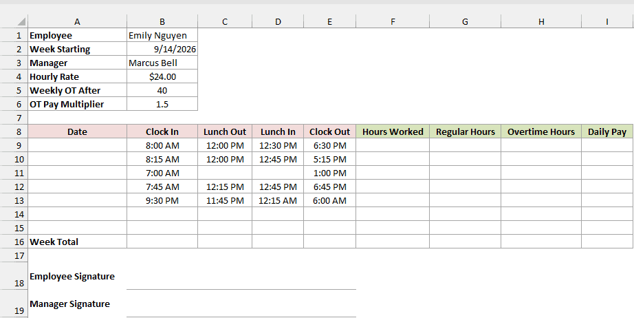
Below is the layout for Emily Nguyen’s week, starting Monday, September 14, 2026.
A1:B6 is the header block: employee, week starting date, manager, hourly rate ($24.00), weekly overtime threshold (40 hours), and overtime pay multiplier (1.5).
Row 8 holds the column headers. Emily’s clock times are typed into B9:E13 as normal times like 8:00 AM. Saturday and Sunday are her days off.
The green headers mark the formula columns, which are still empty. The signature lines for Emily and her manager sit at the bottom.
Instead of typing seven dates, let Excel fill them in from the week starting date in B2. Enter this formula in A9:
=SEQUENCE(7,1,B2)
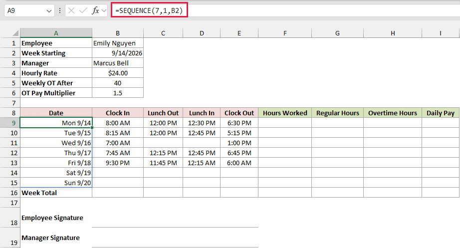
SEQUENCE returns a list of numbers: 7 rows, 1 column, starting at the date in B2 and going up by one.
Dates are numbers in Excel, so that gives you Monday to Sunday.
I formatted A9:A15 with the custom number format ddd m/d, so each date shows its weekday, like Mon 9/14. Next week, change B2 and all seven dates update.
SEQUENCE works in Excel 2021, Excel 2024, and Microsoft 365. In older versions, enter =B2 in A9 and =A9+1 in A10, then copy A10 down to A15.
Next, make sure only real times go into the clock columns.
A time typed as 8:30am (no space) looks fine, but Excel keeps it as text and the formulas can’t use it.
Here are the steps to add a Data Validation rule to the clock times:
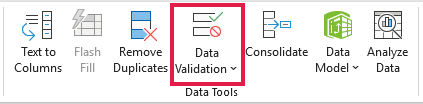
- Select B9:E15, go to the Data tab, and click Data Validation in the Data Tools group.
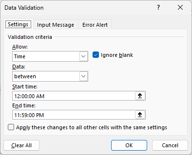
- On the Settings tab, set Allow to Time and Data to between. Enter 12:00 AM as the Start time and 11:59 PM as the End time.
- On the Error Alert tab, keep the Stop style, enter a title and a message (I used “Enter a clock time” and “Type a time such as 8:30 AM or 5:15 PM.”), and click OK.
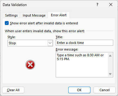
Now Excel rejects anything in B9:E15 that isn’t a clock time, including text like 8:30am and numbers like 830.
Step 2: Calculate Hours Worked (With Lunch Breaks)
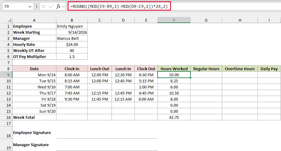
Hours worked is the time between Clock In and Clock Out, minus the lunch break. Enter this formula in F9, then copy it down to F15:
=ROUND((MOD(E9-B9,1)-MOD(D9-C9,1))*24,2)
How does this formula work?
Excel stores a time as a fraction of a day, so 12:00 PM is 0.5. E9-B9 is the length of the shift as a fraction of a day.
MOD(E9-B9,1) uses the MOD function to handle shifts that end after midnight.
On Friday, Emily works 9:30 PM to 6:00 AM, so E13-B13 is negative, and MOD turns it into the correct 8.5 hours.
MOD(D9-C9,1) does the same for the lunch break. Friday needs it too, because Emily’s lunch runs from 11:45 PM to 12:15 AM.
Subtracting the lunch leaves the time worked, and multiplying by 24 turns a fraction of a day into hours. Friday comes out to 8.00.
Blank cells count as zero, so a day with no lunch (Wednesday) or no shift at all (the weekend) still works.
F16 adds up the week with =SUM(F9:F15), which returns 42.75.
I’m copying this formula down instead of using one spilling formula. Each row stays independent, so you can fix a single day, and the sheet works in every Excel version.
Note: ROUND(…,2) cleans up tiny leftovers from how Excel stores times. Without it, Wednesday’s 7:00 AM to 1:00 PM shift is stored as 5.999999999999998 instead of 6, and an exact lookup for 6 hours won’t find it.
Step 3: Split Regular and Overtime Hours
In this example, overtime starts after 40 hours in a week, the number in B5. Regular hours have to stop once the week’s running total reaches 40.
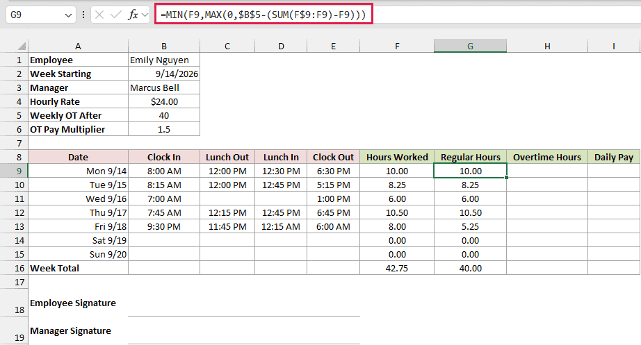
Enter this formula in G9 and copy it down to G15:
=MIN(F9,MAX(0,$B$5-(SUM(F$9:F9)-F9)))
How does this formula work?
SUM(F$9:F9) adds up every hour from Monday down to the current row. Subtracting F9 leaves the hours worked before today.
$B$5 minus that is how much of the 40 hours is still left. MAX(0,…) keeps it from going negative once all 40 are used.
MIN then takes the smaller of today’s hours and what’s left. Emily has 34.75 hours before Friday, so only 5.25 of Friday’s 8 hours count as regular.
Overtime is whatever is left over. Enter this formula in H9 and copy it down to H15:
=F9-G9
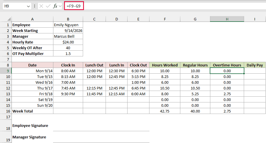
Friday’s shift gives 2.75 overtime hours, which is also the week’s total in H16. Regular hours add up to exactly 40.00 in G16.
The 40 in B5 is just a setting. Overtime rules depend on your employer and where you work, so change it to match yours.
Step 4: Calculate Daily and Weekly Pay
Pay is regular hours at the hourly rate, plus overtime hours at the rate times the multiplier. Enter this formula in I9 and copy it down to I15:
=G9*$B$4+H9*$B$4*$B$6
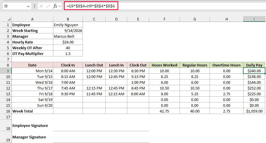
$B$4 is the $24.00 rate and $B$6 is the 1.5 multiplier, so each overtime hour pays $36.00. Friday comes to $225.00: 5.25 hours at $24 plus 2.75 hours at $36.
The week’s pay in I16 is $1,059.00. The rate, threshold, and multiplier all live in the header block, so you only ever change them in one place.
Step 5: Set Up the Timesheet for Printing
A timesheet usually gets printed and signed, so set it up to fit on one page.
Here are the steps:
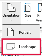
- On the Page Layout tab, click Orientation and choose Landscape.
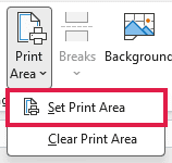
- Select A1:I19. On the Page Layout tab, click Print Area and choose Set Print Area.
- Go to File > Print. Under Settings, open the scaling drop-down and choose Fit Sheet on One Page.
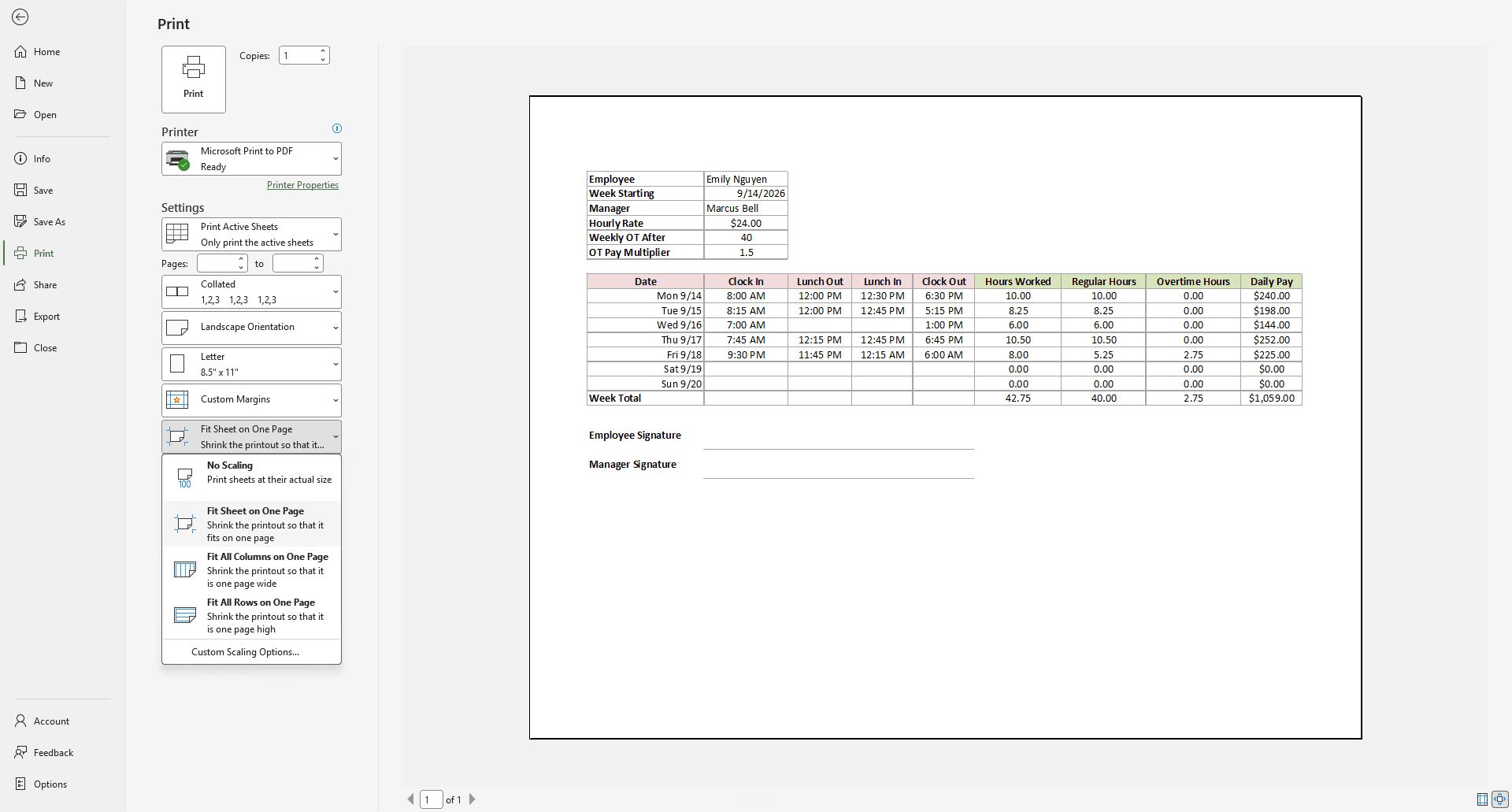
The print preview now shows the header block, the whole week, and both signature lines on one page.
Method #2: Using a Break Duration Column
Some people don’t record when lunch started and ended. They just write down how long it was, and this version works with that.
Below I have Emily’s week again. Clock In and Clock Out are in columns B and C, and column D has the break length in minutes.
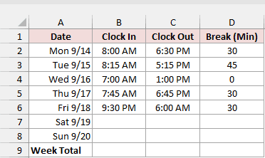
Enter this formula in E2 and copy it down to E8:
=ROUND(MOD(C2-B2,1)*24-D2/60,2)
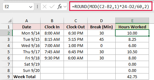
How does this formula work?
MOD(C2-B2,1)*24 is the shift length in hours, and MOD handles Friday’s overnight shift the same way it does in Method #1. D2/60 turns the break minutes into hours.
The results match Method #1 exactly, with 42.75 hours for the week in E9. From there, the regular hours, overtime, and pay formulas work the same way.
Method #3: Using an Excel Timesheet Template
If you’d rather not build anything, Excel has ready-made timesheet templates you can fill in.
Here are the steps:
- Open Excel and go to File > New.
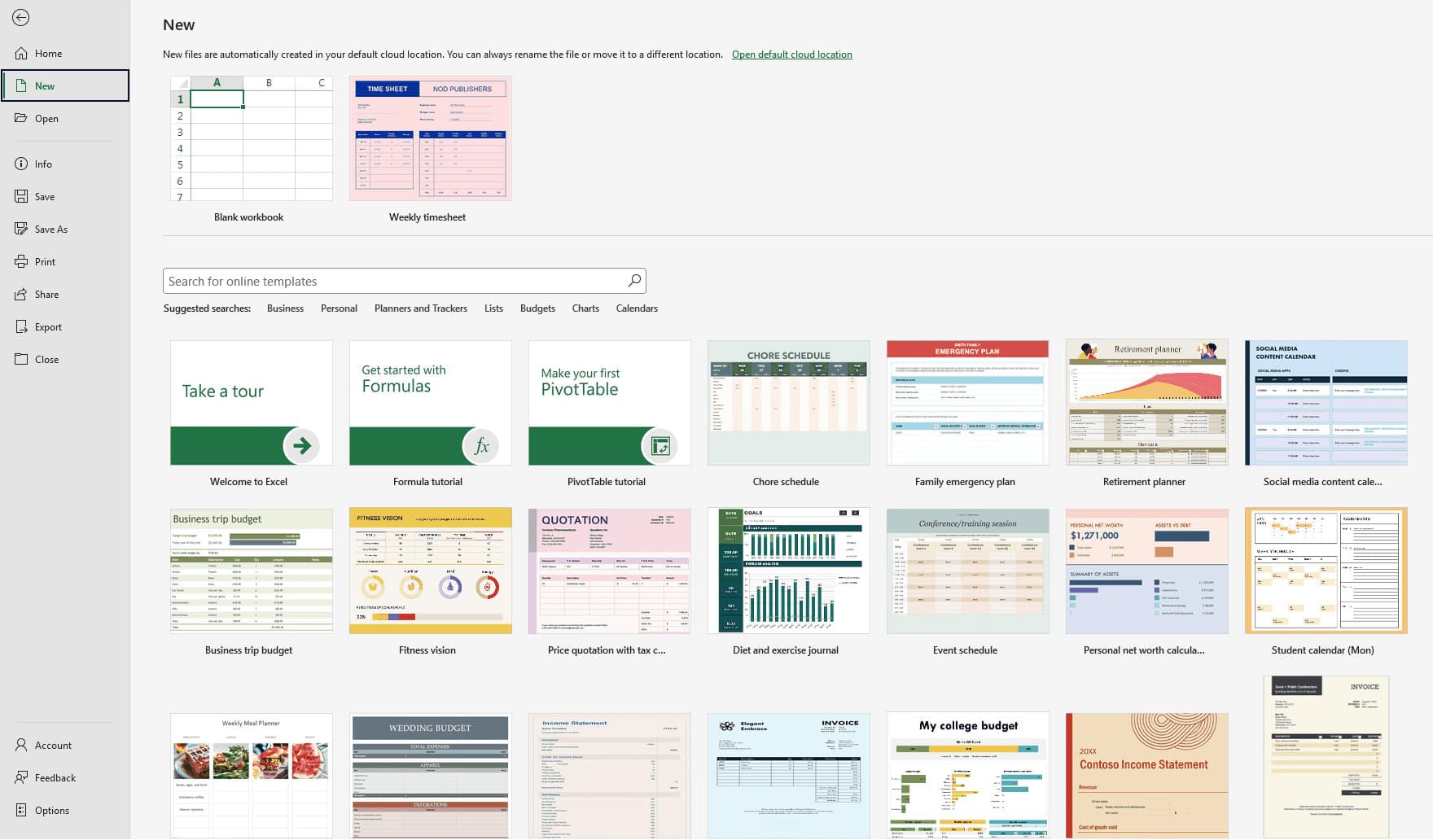
- Type timesheet in the search box and press Enter.
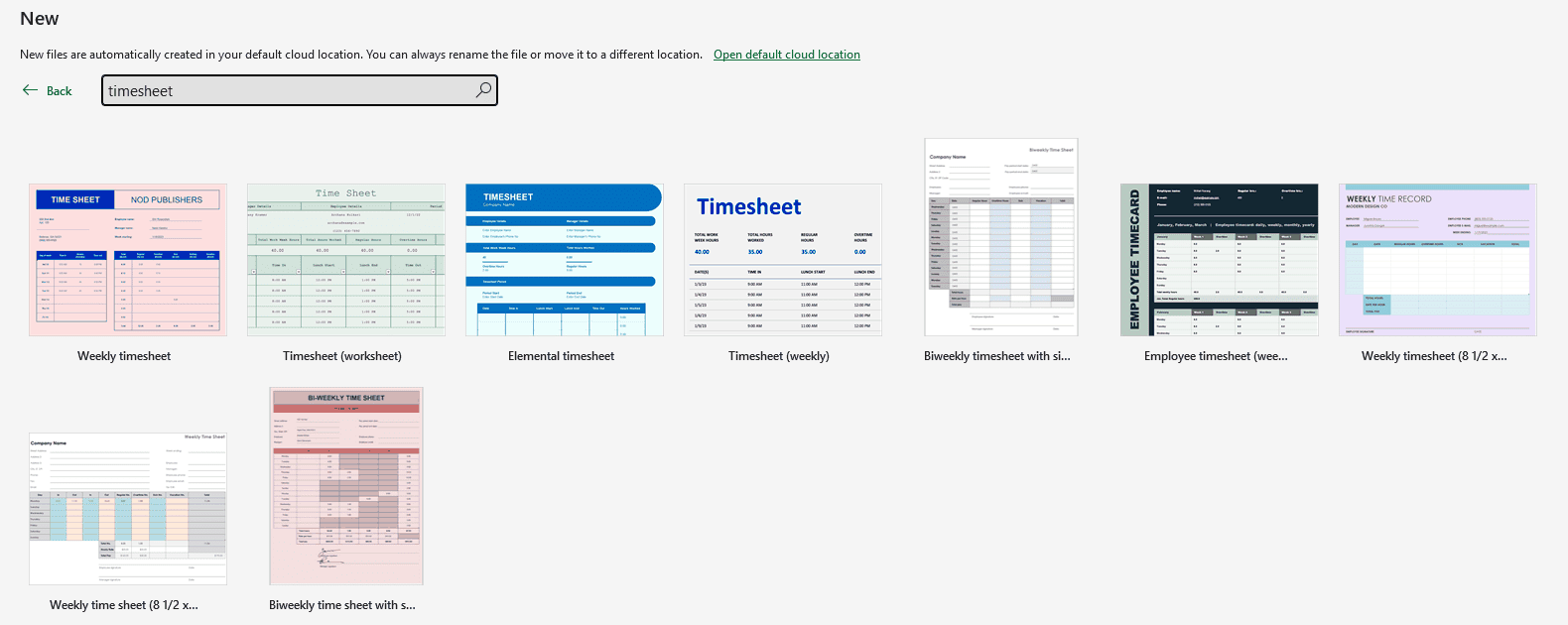
- Click a template to preview it, then click Create.
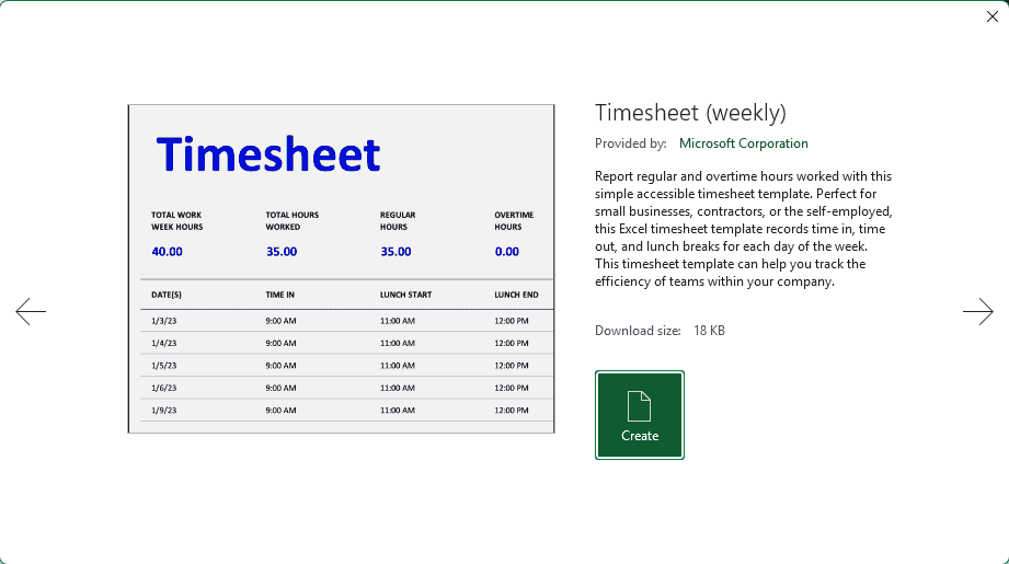
Replace the sample names and times with your own. Before you rely on it, test a shift that crosses midnight and check how the template counts overtime.
Showing Hours Worked as hh:mm Instead of Decimals
The timesheet above returns decimal hours like 10.50, because that’s what a pay formula needs.
If you’d rather see 10:30, keep the result as a time and change how it’s displayed.
Below I have Emily’s week with just the clock times: Clock In, Lunch Out, Lunch In, and Clock Out.
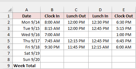
Enter this formula in F2 and copy it down to F8. It’s the Method #1 formula without the *24 and ROUND:
=MOD(E2-B2,1)-MOD(D2-C2,1)
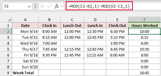
The daily values look right, but the total in F9 (=SUM(F2:F8)) shows 18:45. Emily worked 42 hours and 45 minutes.
The h:mm format starts over every time it passes 24 hours, so 42:45 shows up as 18:45.
Here are the steps to fix the display:
- Select F2:F9 and press Ctrl+1. Pick Custom in the Category list, type [h]:mm in the Type box, and click OK.
![Format Cells dialog with the Custom category and the [h]:mm number format.](https://spreadsheetplanet.com/wp-content/uploads/2026/09/hm-format-cells-custom.png)
The square brackets tell Excel to keep counting hours past 24, so the total now shows 42:45.
![Hours worked in [h]:mm format with the week total showing 42:45.](https://spreadsheetplanet.com/wp-content/uploads/2026/09/hm-result.png)
To use these values for pay, convert them to decimal hours by multiplying by 24. For example, =F9*24 returns 42.75.
Note: Don’t use =TEXT(F2,”h:mm”) to show hours and minutes. TEXT returns text, so a SUM over those cells returns 0 and any pay formula built on them breaks.
Calculating Daily and Weekly Overtime Together
Some employers pay overtime for hours over 8 in a day as well as over 40 in a week.
The tricky part is not paying the same hour as overtime twice.
Below I have Emily’s daily hours from the timesheet in column B, with the week’s 42.75 total in B9.
B11 holds the daily limit (8) and B12 the weekly limit (40).
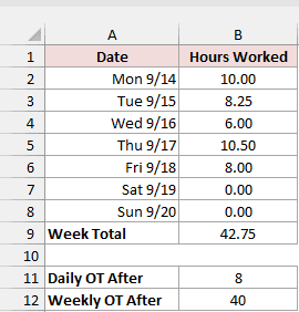
First, the daily overtime. Enter this formula in C2 and copy it down to C8:
=MAX(0,B2-$B$11)
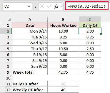
Anything over 8 hours in a day is daily overtime. Monday gives 2.00, Tuesday 0.25, and Thursday 2.50, for 4.75 hours in C9.
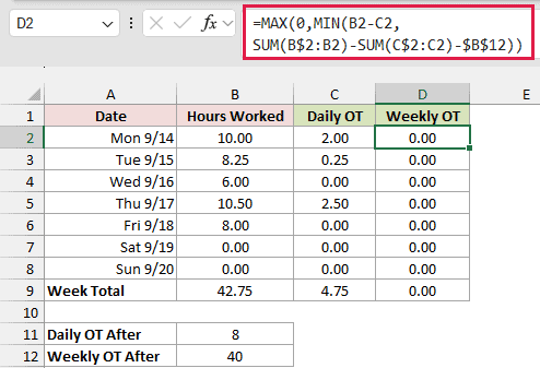
Next, the weekly overtime, counting only hours that weren’t already daily overtime. Enter this formula in D2 and copy it down to D8:
=MAX(0,MIN(B2-C2,SUM(B$2:B2)-SUM(C$2:C2)-$B$12))
How does this formula work?
SUM(B$2:B2)-SUM(C$2:C2) is the hours worked so far this week, minus the daily overtime so far. Only the part above 40 counts as weekly overtime.
MIN caps it at today’s hours that aren’t already daily overtime (B2-C2), and MAX(0,…) keeps it from going negative.
For Emily, that running total never passes 40. Once the 4.75 daily overtime hours come out, she has 38 hours left, so Weekly OT stays at 0.00 all week.
That’s the double counting this formula avoids. A weekly rule on all 42.75 hours would add 2.75 more overtime hours, for 7.5 in total instead of 4.75.
Finally, regular hours are whatever is left. Enter this formula in E2 and copy it down to E8:
=B2-C2-D2
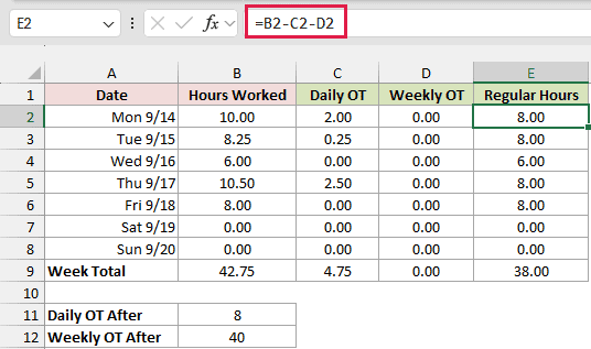
Emily ends up with 38.00 regular hours and 4.75 overtime hours (C9 plus D9). With only the weekly rule from Method #1, she’d get 2.75 overtime hours.
To calculate pay, use the Step 4 formula from Method #1 with Daily OT plus Weekly OT as the overtime hours.
Additional Notes About Creating a Timesheet in Excel
- Keep clock times as real time values. Text that only looks like a time breaks every formula, which is why the Data Validation rule in Step 1 is worth adding.
- The 40-hour weekly threshold, the 8-hour daily limit, and the 1.5 multiplier are example settings. Use the rules that apply to your employer and location.
- The MOD formulas treat an earlier clock-out time as the next day. They can’t handle a single shift of 24 hours or longer.
- For paid time off, put PTO or holiday hours in their own column and pay them at the regular rate. In this setup, keeping them out of Hours Worked means they don’t count toward overtime.
- To stop people from editing the formulas, unlock B9:E15 (Format Cells > Protection > clear Locked), then go to Review > Protect Sheet.
Frequently Asked Questions
Here are answers to a few common questions about building a timesheet in Excel.
How do I enter AM and PM times in Excel?
Type a space before AM or PM, like 8:30 AM. A short 9:30 p also works, and so does 24-hour time like 17:30.
Without the space (8:30am), Excel keeps the entry as text, and the Data Validation rule from Step 1 rejects it.
How do I make a biweekly or monthly timesheet?
Make one copy of the weekly sheet per week. Right-click the sheet tab, choose Move or Copy, tick Create a copy, and then change the week starting date.
Each copy keeps its own 40-hour count, so weekly overtime stays correct. A summary sheet can then add up each week’s totals from row 16.
How do I round clock-in times to the nearest 15 minutes?
MROUND can round a time to the nearest quarter hour when you give it “0:15″ as the multiple, like =MROUND(B9,”0:15”).
A clock-in at 8:07 AM rounds to 8:00 AM, and 8:08 AM rounds to 8:15 AM.
How do I add the current time without it changing later?
Press Ctrl+Shift+; (semicolon) to enter the current time as a fixed value. On a Mac, press Command+; instead.
Don’t use NOW() for clock punches. It recalculates every time the workbook changes, so yesterday’s clock-in would keep moving.
Can I track several employees in one workbook?
Yes, but give each employee their own sheet. The regular-hours formula adds up every row above it, so it assumes every row belongs to one person.
Conclusion
In this article, I showed you how to build a weekly timesheet in Excel with lunch breaks, overnight shifts, overtime, pay, and a one-page print setup.
I also covered a break-duration version, Excel’s timesheet templates, hh:mm totals, and daily plus weekly overtime.
For most people, the formula timesheet in Method #1 is the one to start with.
I hope you found this article helpful.
Other Excel articles you may also like:
