
Excel’s MROUND function rounds a number to the nearest multiple you specify.
Use it for quantities sold in packs or times rounded to fixed intervals. The number and multiple must have the same sign.
Inputs must be numeric. Text that cannot be interpreted as a number can produce a #VALUE! error.
In this article, I’ll show you how to round prices and time to set multiples, compare rounding functions, and handle negative inputs.
MROUND Function Syntax in Excel
The MROUND function rounds a number to the nearest multiple you specify.
=MROUND(number, multiple)
- number (required) is the value you want to round.
- multiple (required) is the multiple to which you want to round the number.
MROUND compares the remainder with half the multiple. It rounds away from zero when the remainder is at least half the multiple.
When to Use MROUND Function
- Round prices or estimates to practical increments such as $5, $10, or $100.
- Round cash amounts to the nearest nickel or another currency increment.
- Round elapsed times to billing intervals such as 15 or 30 minutes.
- Place weights, quantities, or measurements into their nearest standard bracket.
- Round mixed positive and negative values after matching the sign of each multiple.
Example 1: Round Prices to the Nearest $5
Let’s start with a straightforward pricing example.
Below is the dataset. Column A lists home-service jobs, column B contains raw estimates, and column C will hold the quoted prices.
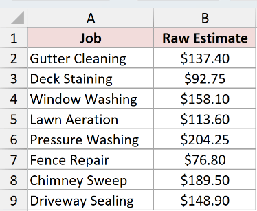
We want to round each raw estimate to the nearest $5.
Here is the formula entered in C2 and copied down the column:
=MROUND(B2,5)
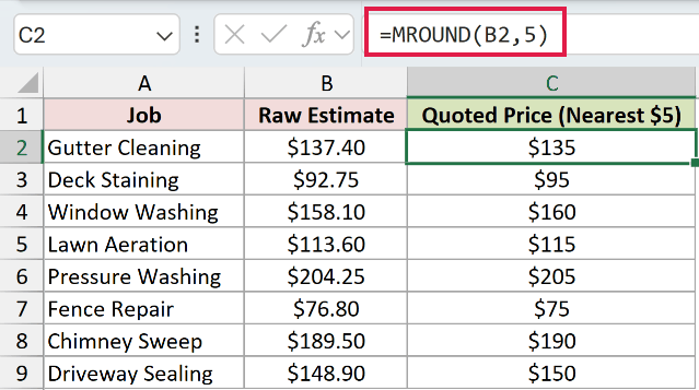
The formula uses the estimate in B2 as the number and 5 as the multiple.
The $137.40 gutter-cleaning estimate becomes $135. The $92.75 deck-staining estimate becomes $95, while the $204.25 pressure-washing estimate becomes $205.
This changes the stored value. Applying a number format would only change how the original estimate looks.
Example 2: Round Cash to the Nearest Nickel
Here’s a useful example for cash transactions.
Below is the dataset. It contains receipt numbers, amounts due, cash-rounded totals, and the difference caused by rounding.
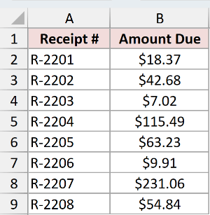
We want to round each amount to the nearest $0.05 and measure the change.
Here is the cash-rounding formula entered in C2 and copied down:
=MROUND(B2,0.05)
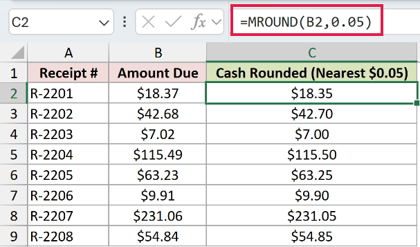
The multiple 0.05 tells Excel to use nickel increments. The $18.37 amount becomes $18.35, while $42.68 becomes $42.70.
To see the effect of rounding, enter this formula in D2 and copy it down:
=ROUND(MROUND(B2,0.05)-B2,2)
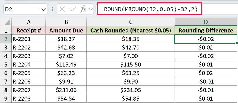
The inner MROUND calculates the cash total. The formula subtracts the original amount, then ROUND keeps the difference to two decimal places.
Receipt R-2201 has a difference of -$0.02. Receipt R-2202 has a difference of $0.02, and R-2208 has a difference of $0.01.
Example 3: Round Time to 15 or 30 Minutes
Now let’s round logged time to common billing intervals.
Below is the dataset. Column B contains each duration, while columns C and D will show the nearest 15-minute and 30-minute values.
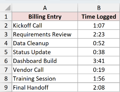
We want to compare quarter-hour and half-hour rounding for every billing entry.
Here is the 15-minute formula entered in C2 and copied down:
=MROUND(B2,TIME(0,15,0))
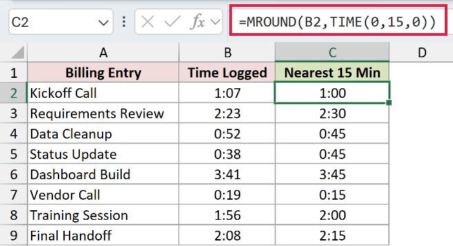
TIME creates a 15-minute Excel time value for the multiple. The 1:07 kickoff call becomes 1:00, and the 2:23 requirements review becomes 2:30.
Here is the 30-minute formula entered in D2 and copied down:
=MROUND(B2,1/48)
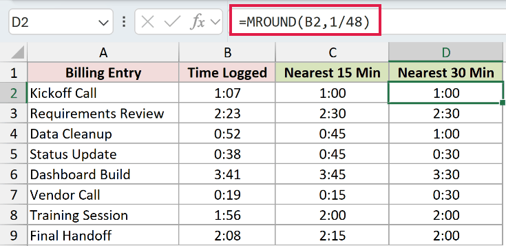
Excel stores time as a fraction of a day. Because a day contains 48 half-hours, 1/48 represents 30 minutes.
The 0:52 data-cleanup entry becomes 1:00. The 3:41 dashboard-build entry becomes 3:30, while the 1:56 training session becomes 2:00.
Pro Tip: Use a time value as the multiple. For 15 minutes, TIME(0,15,0), 1/96, and "0:15" all represent the interval. The result cells also need a time format such as h:mm.
Example 4: Compare MROUND, CEILING.MATH, and FLOOR.MATH
This comparison makes the rounding direction easier to see.
Below is the dataset. It lists shipment weights and three result columns that round each weight to a 50-pound bracket.
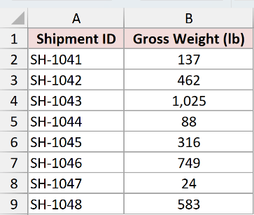
We want to compare nearest, upward, and downward rounding on the same shipments.
Here is the MROUND formula entered in C2 and copied down:
=MROUND(B2,50)
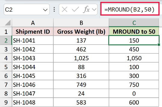
MROUND chooses the closest multiple of 50. A weight of 137 becomes 150, while 462 becomes 450.
The 24-pound shipment returns 0 with MROUND because 0 is its nearest multiple of 50.
Here is the CEILING.MATH formula entered in D2 and copied down:
=CEILING.MATH(B2,50)
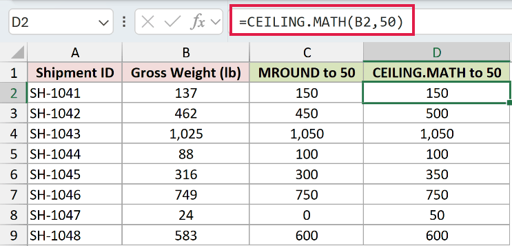
CEILING.MATH always rounds these positive weights upward. The 462-pound shipment becomes 500, and the 316-pound shipment becomes 350.
CEILING.MATH returns 50 for the 24-pound shipment because it always rounds upward.
Here is the FLOOR.MATH formula entered in E2 and copied down:
=FLOOR.MATH(B2,50)
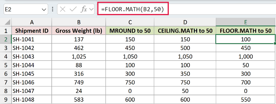
FLOOR.MATH rounds the weights downward. The 1,025-pound shipment becomes 1,000, while the 583-pound shipment becomes 550.
Pro Tip: Use CEILING.MATH when a freight or material quantity must cover the full requirement. MROUND can choose a lower bracket, including 0, because distance rather than direction controls its result.
Example 5: Fix #NUM! for Negative Numbers
Mixed positive and negative values expose MROUND’s most common error.
Below is the dataset. Column B contains budget variances, column C shows regular MROUND results, and column D provides sign-safe results.
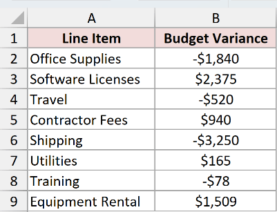
We want to round every variance to the nearest $100 without losing the negative rows.
First, enter the regular formula in C2 and copy it down:
=MROUND(B2,100)
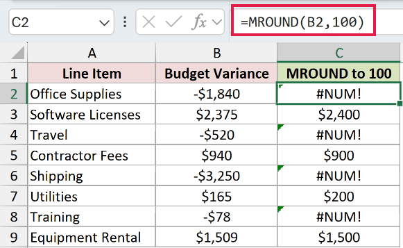
MROUND requires the number and multiple to have the same sign.
The negative variances in B2, B4, B6, and B8 make C2, C4, C6, and C8 return #NUM!.
Positive rows still calculate. The $2,375 software-license variance becomes $2,400, while the $940 contractor-fee variance becomes $900.
To handle both signs, enter this formula in D2 and copy it down:
=MROUND(B2,SIGN(B2)*100)
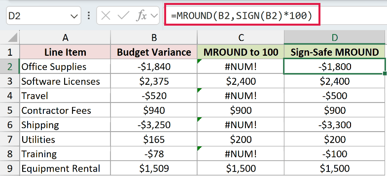
SIGN returns 1 for a positive number and -1 for a negative number. Multiplying by 100 gives MROUND a multiple with the correct sign.
The -$1,840 office-supplies variance becomes -$1,800. The -$3,250 shipping variance becomes -$3,300, and the -$78 training variance becomes -$100.
Pro Tip: Another sign-safe option is =SIGN(B2)*MROUND(ABS(B2),100). Avoid hiding the error with IFERROR, because that removes the result instead of correcting the mismatched signs.
Example 6: Understand Exact Halves and Decimal Multiples
Finally, let’s look closely at how MROUND chooses between two multiples.
Below is the dataset. Each row supplies a number, its own multiple, and a result column for comparing several rounding cases.
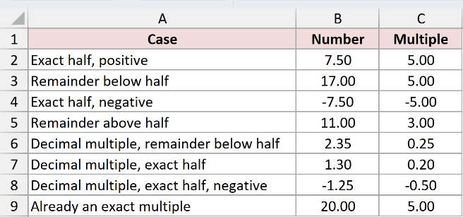
We want to see how remainders, exact halves, decimal multiples, and exact matches behave.
Here is the formula entered in D2 and copied down:
=MROUND(B2,C2)
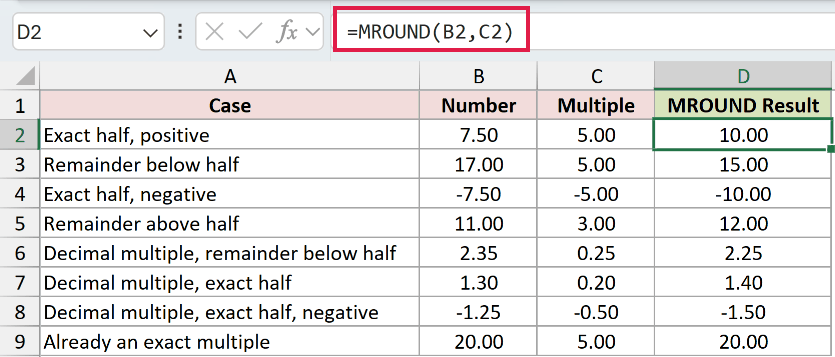
The formula reads both arguments from the current row, so each case can use a different number and multiple.
An exact half rounds away from zero. The positive 7.50 becomes 10.00, while -7.50 with a -5.00 multiple becomes -10.00.
A remainder below half rounds toward the closer multiple. The 17.00 value becomes 15.00, and 2.35 with a 0.25 multiple becomes 2.25.
Microsoft documents the decimal midpoint 1.30 with a 0.20 multiple returning 1.40. The Tips section explains why you should not treat this result as a general rule.
The negative case uses -1.25 and -0.50 and returns -1.50.
When the number is already a multiple, MROUND leaves it unchanged. The 20.00 value with a 5.00 multiple returns 20.00.
Tips & Common Mistakes
- MROUND is one of the few math functions that never spills. The MAP and LAMBDA functions in
=MAP(B2:B9,LAMBDA(x,MROUND(x,5)))are Microsoft 365 only. Filling down works in every Excel version that has MROUND. - Keep the number and multiple signs the same. A positive multiple paired with a negative number returns #NUM!, so use SIGN or ABS to correct the cause.
- Microsoft says MROUND’s rounding direction is undefined for midpoint numbers when the multiple is decimal. For more predictable midpoint control, use
=ROUND(number/multiple,0)*multiple. - Use MROUND when you need the nearest multiple. Use ROUND when the target is a fixed number of decimal places.
- Enter a time interval as an Excel time value, not as a whole minute count. Entering 15 means 15 days, not 15 minutes.
- MROUND returns #VALUE! when either argument is non-numeric. Check imported values that look like numbers but are stored as text.
- For prices ending in .99, round to the nearest whole number and subtract one cent with
=MROUND(A2,1)-0.01.
MROUND is a good fit whenever the target is an increment rather than a decimal place.
Use it for prices, cash, times, and measurements, but remember its sign rule and its refusal to accept array input.
Related Excel Functions / Articles:
