Chi-Square measures how far observed values differ from expected values. It tells you whether the difference is real or just a random chance.
In Excel, you can calculate the Chi-Square value in three steps using the CHISQ.TEST function.
CHISQ.TEST calculates the p-value (probability value) for a Chi-Square test.
CHISQ.TEST Syntax
CHISQ.TEST(actual_range,expected_range)
It takes two arguments:
- actual_range – the range with your observed values.
- expected_range – the range with the values you’d expect if there were no relationship.
Example: Calculating Chi-Square Value in Excel
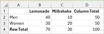
Let’s say you ran a survey to check if men and women prefer different drinks and collected this data:
| Gender | Lemonade | Milkshake | Total |
|---|---|---|---|
| Men | 40 | 10 | 50 |
| Women | 30 | 20 | 50 |
| Total | 70 | 30 | 100 |
You want to know if drink preference depends on gender.
Step 1: Enter the Observed Values in Excel
Enter the observed values in cell range B2:C3.
Step 2: Calculate Expected Values
Calculate the expected values using this formula:
Expected Value = Row Total x Column Total / Grand TotalCalculate these for each gender in cell range G2:H3.
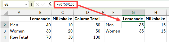
In this example, we’re testing whether two variables (gender and drink preference) are independent.
So the expected values are calculated from the observed totals using a formula.
The idea is, if there is no relation between the drink and the gender, of the 70 people surveyed for lemonade, 35 men and 35 women would prefer lemonade, and out of the 30 people who preferred milkshake, 15 men and 15 women would prefer milkshake.
In other cases, you might already have expected values from past data or a known benchmark (for example, “last year 60% chose Lemonade and 40% chose Milkshake”). In that situation, you’d skip Step 2 and directly use your existing expected values in the CHISQ.TEST function.
Step 3: Calculate the Chi-Square
Use the CHISQ.TEST function:
=CHISQ.TEST(B2:C3,G2:H3)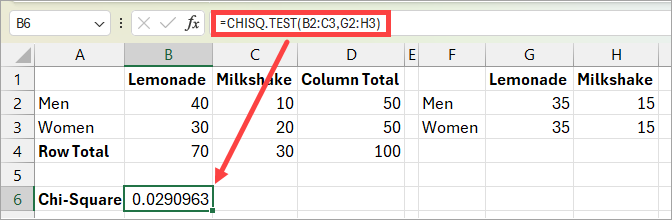
The above formula returns 0.0290963.
Since this is less than 0.05, the result is statistically significant, which means the drink preference is related to gender.
If the value had been 0.05 or higher, the result wouldn’t be significant, meaning drink preference has nothing to do with gender.
So this is how you can use an inbuilt function in Excel to calculate chi-square value.
I hope you found this article helpful.
Other Excel articles you may also like: