Most people use spreadsheets software such as Microsoft Excel to process their data and carry out their analysis tasks.
When performing an analysis of data, a number of statistical metrics come into play. Some of these include the means, the medians, standard deviations, and standard errors. These metrics help in understanding the true nature of the data.
In this article, I will show you two ways to calculate the Standard Error in Excel.
One of the methods involves using a formula and the other involves using a Data Analytics Tool Pack that usually comes with every copy of Excel.
So let’s get started!
What is Standard Error?
When working with real-world data, it is often not possible to work with data of the entire population. So we usually take random samples from the population and work with them.
The standard error of a sample tells how accurate its mean is in terms of the true population mean.
In other words, the standard error of a sample is its standard deviation from the population mean.
This helps analyze how accurately your sample’s mean represents the true population. It also helps analyze the amount of dispersion or variation between your different data samples.
Also see: Standard Error Calculator
How is Standard Error Calculated?
The Standard Error for a sample is usually calculated using the formula:
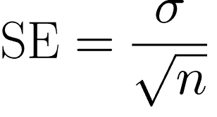
In this above formula:
- SE is Standard Error
- σ represents the Standard deviation of the sample
- n represents the sample size.
Also read: Calculate the Interquartile Range in Excel?
How to Find the Standard Error in Excel Using a Formula
Unfortunately, unlike the Standard Deviation, Excel does not have a built-in formula to calculate the Standard Error, at least not at the time of writing this tutorial.
However, you could use the above formula to easily and quickly calculate the standard error. Here are the steps you need to follow:
- Click on the cell where you want the Standard Error to appear and click on the formula bar next to the fx symbol just below your toolbar.
- Type the symbol ‘=’ in the formula bar. And type: =STDEV(
- Drag and select the range of cells that are part of your sample data. This will add the location of the range in your formula. So, if your sample data is in cells B2 to B14, you will see: =STDEV(B2:B14 in the formula bar.
- Close the bracket for the STDEV formula. So far, you have used the STDEV function to find the Standard deviation of your sample data.
- Next, we want to divide this Standard deviation by the square root of the sample size. So let’s continue with our formula. Click on the formula bar after the closing brackets of the STDEV formula and add a ‘/’ symbol to indicate that you want to divide the result of the STDEV function. So your formula so far is: =STDEV(B2:B14)/
- To find the square root of a number, we use the SQRT formula. So next, type SQRT(. Your formula bar will now have the formula: =STDEV(B2:B14)/SQRT(
- Finally, you want the sample size. For this, you need to use the COUNT function. So, type COUNT( after what you already have in your formula bar. Again, drag and select the range of cells that are part of your sample data and close the bracket for the COUNT formula. This will give you the number of cells in your selected range.
- Close the bracket for the SQRT function too. So your final formula should look like this: =STDEV(B2:B14)/SQRT(COUNT(B2:B14)) Notice there are two closing braces in the end. One is for the COUNT function, the other is for the SQRT function.
- That’s it! Press the return key on your keyboard and you got your sample’s Standard Error!
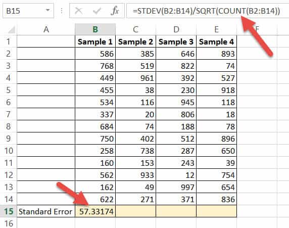
To find the Standard errors for the other samples, you can apply the same formula to these samples too.
If your samples are placed in columns adjacent to one another (as shown in the above image), you only need to drag the fill handle (located at the bottom left corner of your calculated cell) to the right.
This will copy the same formula to all the other cells on the right, and you will get standard errors for each of your samples!
Also read: How to Calculate Variance in Excel?
How to Find the Standard Error in Excel Using the Data Analysis Toolpak
If you’re not in the mood to type complex formulae, there’s an easier way to find not just the Standard error, but practically all the statistical metrics you might need to analyze your sample data.
For this, you will need to install the Data Analysis Toolpak. This package gives you access to a variety of statistical functions, which include correlation functions, z-test, and t-test functions too.
Once you install the package, you can use the tool whenever you need to analyze data, without having to re-install it each time.
The Data Analysis Toolpak is free to use and comes along with your Excel package, but for simplicity, it does not appear in your standard toolbar. You need to activate it in order for it to be added to your toolbar.
The process of activating it is quite simple. Just follow these steps to install and activate your Data Analysis Toolpak:
- Click the File tab and click on Options. This will open the Options window for you.
- From here, click “Add-ins” from the left sidebar.
- From the list of Add-ins, select Analysis ToolPak.
- At the bottom of the window, click on the ‘Go’ button just next to Manage: Add-ins.
- Click the checkmark for Analysis ToolPak and click OK.
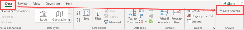
With this, your Data Analysis Toolpak will get added to your Excel Toolbar. When you click the Excel ‘Data’ tab, you should find a tool named “Data Analysis” at the far right of the Data toolbar (under the ‘Analysis’ group).
Now, to find out your Standard Error and other Statistical metrics, do the following:
- Click on the Data Analysis tool under the Data tab. This will open the Analysis Tools dialog box.
- Select “Descriptive Statistics” from the list on the left of the dialog box and click OK.
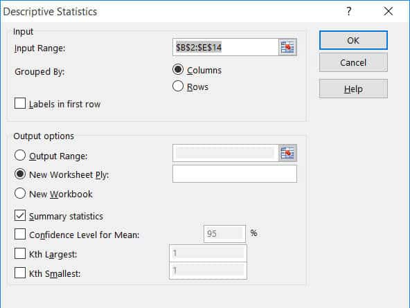
- Enter the location of the range of cells that contain your sample data into the “Input Range” box. You can also choose to drag and select the range of cells that you need too. If you have data for more than one sample arranged in adjacent columns, you can select the data in all the columns. You will get your results separately for each column.
- If your data has column headers, check the “Labels in first row” box.
- Select where you want your results to be displayed. It is safer to select “New Worksheet”. This will ensure that the details get displayed on a newly created worksheet, and will not disturb any data on your current worksheet.
- Select the checkbox next to “Summary Statistics” and click OK.
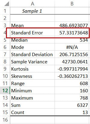
This will display all your analytical metrics in a new worksheet.
These metrics will also include the Standard Error for your selected sample data. If you had selected multiple data sets in multiple columns, you will get analytics for each column separately.
Also read: Calculate Correlation Coefficient in Excel
Conclusion
In this article, we discussed two ways in which you can find the Standard error for your sample data.
You can either create a formula to calculate it or use a data analytics tool, like the Data Analysis Toolpak that comes with Excel.
Either way, you will be able to use the Standard error information to analyze your sample data for further processing.
Hope you found this Excel tutorial useful!
Other Excel tutorials you may find useful:
- How to Convert Decimal to Fraction in Excel
- How to Square a Number in Excel
- How to Subtract Multiple Cells from One Cell in Excel
- How to Find Range in Excel
- How to Find Outliers in Excel
- How to Calculate IRR with Excel
- How to Calculate NPV in Excel (Net Present Value)
- How to Calculate Confidence Interval in Excel
- How to Get the p-Value in Excel?
- How to Find Z-score in Excel?
- How to Calculate Percentage Difference in Excel
- Calculate the Coefficient of Variation in Excel
- How to Calculate Mean Squared Error (MSE) in Excel?
- Calculate Coefficient of Determination in Excel
- Calculate CHI-SQUARE in Excel